Analyzing PBMC scATAC-seq
Compiled: March 20, 2026
Source:vignettes/pbmc_vignette.Rmd
pbmc_vignette.RmdFor this tutorial, we will be analyzing a single-cell ATAC-seq dataset of human peripheral blood mononuclear cells (PBMCs) provided by 10x Genomics. The following files are used in this vignette, all available through the 10x Genomics website:
- The Raw
data
- The Metadata
- The fragments file
- The fragments file index
View data download code
To download all the required files, you can run the following lines in a shell:
wget https://cf.10xgenomics.com/samples/cell-atac/2.1.0/10k_pbmc_ATACv2_nextgem_Chromium_Controller/10k_pbmc_ATACv2_nextgem_Chromium_Controller_filtered_peak_bc_matrix.h5
wget https://cf.10xgenomics.com/samples/cell-atac/2.1.0/10k_pbmc_ATACv2_nextgem_Chromium_Controller/10k_pbmc_ATACv2_nextgem_Chromium_Controller_singlecell.csv
wget https://cf.10xgenomics.com/samples/cell-atac/2.1.0/10k_pbmc_ATACv2_nextgem_Chromium_Controller/10k_pbmc_ATACv2_nextgem_Chromium_Controller_fragments.tsv.gz
wget https://cf.10xgenomics.com/samples/cell-atac/2.1.0/10k_pbmc_ATACv2_nextgem_Chromium_Controller/10k_pbmc_ATACv2_nextgem_Chromium_Controller_fragments.tsv.gz.tbi
PBMC scATAC-seq Analysis
When pre-processing chromatin data, Signac uses information from two related input files:
Count matrix. This is analogous to the gene expression count matrix used to analyze single-cell RNA-seq. However, instead of genes, rows of the matrix represents a regions of the genome. Each value in the matrix represents the number of Tn5 integration sites for each single barcode (i.e. a cell) within the region. You can find more detail on the 10X Website.
Fragment file. This represents a full list of all unique fragments across all single cells. It is a substantially larger file, is slower to work with, and is stored on-disk (instead of in memory). However, the advantage of retaining this file is that it contains all fragments associated with each single cell, as opposed to only fragments that map to peaks. More information about the fragment file can be found on the 10x Genomics website or on the sinto website.
In this vignette we demonstrate two approaches for analysing the scATAC-seq data. The first uses a set of peak calls tailored to the dataset, output by Cellranger. This approach tends to work fine, but results in a dataset that is difficult to compare with other data as the feature set is unique to the dataset.
We demonstrate an alternative approach using our recently-released REMO universal scATAC-seq features for the human genome. This enables easier comparisons across datasets through feature standardization, and enables a much more scalable analysis by using a greatly reduced number of features. For more, check out our recent preprint.
This tab demonstrates the standard peak-based analysis workflow using CellRanger-called peaks.
First load Signac, Seurat, and some other packages we will be using for analyzing human data.
library(Signac)
library(Seurat)
library(GenomicRanges)
library(ggplot2)
library(patchwork)
library(GenomeInfoDb)
library(dplyr)
Pre-processing workflow
We start by creating a Seurat object using the count matrix and cell metadata generated by cellranger-atac, and store the path to the fragment file on disk in the Seurat object:
counts <- Read10X_h5(filename = "10k_pbmc_ATACv2_nextgem_Chromium_Controller_filtered_peak_bc_matrix.h5")
metadata <- read.csv(
  file = "10k_pbmc_ATACv2_nextgem_Chromium_Controller_singlecell.csv",
  header = TRUE,
  row.names = 1
)

gr_assay <- CreateGRangesAssay(
  counts = counts,
  fragments = "10k_pbmc_ATACv2_nextgem_Chromium_Controller_fragments.tsv.gz",
  min.cells = 10,
  min.features = 200
)

pbmc <- CreateSeuratObject(
  counts = gr_assay,
  assay = "peaks",
  meta.data = metadata
)
pbmc## An object of class Seurat
## 165434 features across 10246 samples within 1 assay
## Active assay: peaks (165434 features, 0 variable features)
## 1 layer present: countsWhat if I don’t have an H5 file?
If you do not have the .h5 file, you can still run an
analysis. You may have data that is formatted as three files, a counts
file (.mtx), a cell barcodes file, and a peaks file. If
this is the case you can load the data using the
Matrix::readMM() function:
counts <- Matrix::readMM("filtered_peak_bc_matrix/matrix.mtx")
barcodes <- readLines("filtered_peak_bc_matrix/barcodes.tsv")
peaks <- read.table("filtered_peak_bc_matrix/peaks.bed", sep = "\t")
peaknames <- paste(peaks$V1, peaks$V2, peaks$V3, sep = "-")

colnames(counts) <- barcodes
rownames(counts) <- peaknames
Alternatively, you might only have a fragment file. In this case you
can create a count matrix using the FeatureMatrix()
function:
fragpath <- "10k_pbmc_ATACv2_nextgem_Chromium_Controller_fragments.tsv.gz"

# Define cells
# If you already have a list of cell barcodes to use you can skip this step
total_counts <- CountFragments(fragpath)
cutoff <- 1000 # Change this number depending on your dataset!
barcodes <- total_counts[total_counts$frequency_count > cutoff, ]$CB

# Create a fragment object
frags <- CreateFragmentObject(path = fragpath, cells = barcodes)

# First call peaks on the dataset
# If you already have a set of peaks you can skip this step
peaks <- CallPeaks(frags)

# Quantify fragments in each peak
counts <- FeatureMatrix(fragments = frags, features = peaks, cells = barcodes)
The ATAC-seq data is stored using a custom assay, the
GRangesAssay. This enables some specialized functions for
analysing genomic single-cell assays such as scATAC-seq. By printing the
assay we can see some of the additional information that can be
contained in the GRangesAssay, including motif information,
gene annotations, and genome information.
pbmc[["peaks"]]## GRangesAssay data with 165434 features for 10246 cells
## Variable features: 0
## Annotation present: FALSE
## Fragment files: 1
## Motifs present: FALSE
## Links present: 0
## Region aggregation matrices: 0For example, we can call granges on a Seurat object with
a GRangesAssay set as the active assay (or on a
GRangesAssay) to see the genomic ranges associated with
each feature in the object. See the object interaction vignette for more
information about the GRangesAssay class.
granges(pbmc)## GRanges object with 165434 ranges and 0 metadata columns:
## seqnames ranges strand
## <Rle> <IRanges> <Rle>
## [1] chr1 9772-10660 *
## [2] chr1 180712-181178 *
## [3] chr1 181200-181607 *
## [4] chr1 191183-192084 *
## [5] chr1 267576-268461 *
## ... ... ... ...
## [165430] KI270713.1 13054-13909 *
## [165431] KI270713.1 15212-15933 *
## [165432] KI270713.1 21459-22358 *
## [165433] KI270713.1 29676-30535 *
## [165434] KI270713.1 36913-37813 *
## -------
## seqinfo: 35 sequences from an unspecified genome; no seqlengthsWe then remove the features that correspond to chromosome scaffolds e.g. (KI270713.1) or other sequences instead of the (22+2) standard chromosomes.
pbmc <- pbmc[seqnames(pbmc) %in% standardChromosomes(pbmc), ]We can also add gene annotations to the pbmc object for
the human genome. This will allow downstream functions to pull the gene
annotation information directly from the object.
Multiple patches are released for each genome assembly. When dealing with mapped data (such as the 10x Genomics files we will be using), it is advisable to use the annotations from the same assembly patch that was used to perform the mapping.
From the dataset summary, we can see that the reference package 10x Genomics used to perform the mapping was “GRCh38-2020-A”, which corresponds to the Ensembl v98 patch release. For more information on the various Ensembl releases, you can refer to this site.
library(AnnotationHub)
ah <- AnnotationHub()

# Search for the Ensembl 98 EnsDb for Homo sapiens on AnnotationHub
query(ah, "EnsDb.Hsapiens.v98")
## AnnotationHub with 1 record
## # snapshotDate(): 2025-10-29
## # names(): AH75011
## # $dataprovider: Ensembl
## # $species: Homo sapiens
## # $rdataclass: EnsDb
## # $rdatadateadded: 2019-05-02
## # $title: Ensembl 98 EnsDb for Homo sapiens
## # $description: Gene and protein annotations for Homo sapiens based on Ensembl version 98.
## # $taxonomyid: 9606
## # $genome: GRCh38
## # $sourcetype: ensembl
## # $sourceurl: http://www.ensembl.org
## # $sourcesize: NA
## # $tags: c("98", "AHEnsDbs", "Annotation", "EnsDb", "Ensembl", "Gene", "Protein", "Transcript")
## # retrieve record with 'object[["AH75011"]]'
ensdb_v98 <- ah[["AH75011"]]
# extract gene annotations from EnsDb
annotations <- GetGRangesFromEnsDb(ensdb = ensdb_v98)

# change to UCSC style since the data was mapped to hg38
seqlevels(annotations) <- paste0("chr", seqlevels(annotations))
genome(annotations) <- "hg38"
# add the gene information to the object
Annotation(pbmc) <- annotations
Computing QC Metrics
We can now compute some QC metrics for the scATAC-seq experiment. We currently suggest the following metrics below to assess data quality. As with scRNA-seq, the expected range of values for these parameters will vary depending on your biological system, cell viability, and other factors.
Nucleosome banding pattern: The histogram of DNA fragment sizes (determined from the paired-end sequencing reads) should exhibit a strong nucleosome banding pattern corresponding to the length of DNA wrapped around a single nucleosome.
Transcriptional start site (TSS) enrichment score: The ENCODE project has defined an ATAC-seq targeting score based on the ratio of fragments centered at the TSS to fragments in TSS-flanking regions (see https://www.encodeproject.org/data-standards/terms/). Poor ATAC-seq experiments typically will have a low TSS enrichment score.
Total number of fragments: A measure of cellular sequencing depth / complexity. Cells with very few fragments may need to be excluded due to low sequencing depth. Cells with extremely high levels may represent doublets, nuclei clumps, or other artefacts.
Fraction of fragments in promoters: Represents the fraction of all fragments that fall within promoter regions. Cells with low values (i.e. <15-20%) often represent low-quality cells or technical artifacts that should be removed.
Ratio reads in genomic blacklist regions: The ENCODE project has provided a list of blacklist regions, representing reads which are often associated with artefactual signal. Cells with a high proportion of reads mapping to these areas (compared to reads mapping to peaks) often represent technical artifacts and should be removed.
We can compute a range of scATAC-seq QC metrics in Signac using the
ATACqc function:
pbmc <- ATACqc(pbmc)The relationship between variables stored in the object metadata can
be visualized using the DensityScatter() function. This can
also be used to quickly find suitable cutoff values for different QC
metrics by setting quantiles=TRUE:
DensityScatter(pbmc, x = "total_fragments", y = "TSS_enrichment", log_x = TRUE, quantiles = TRUE)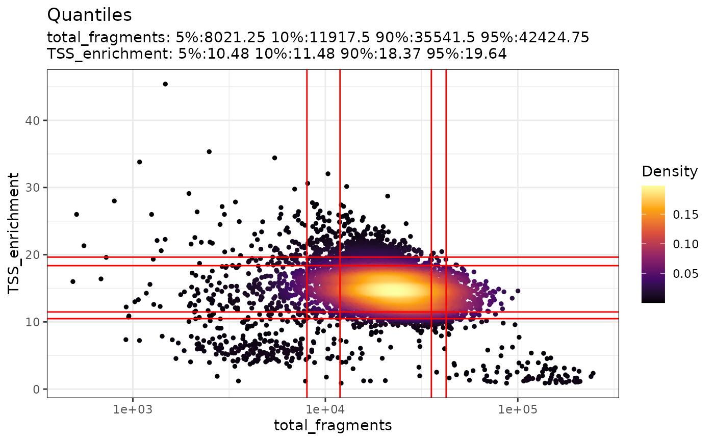
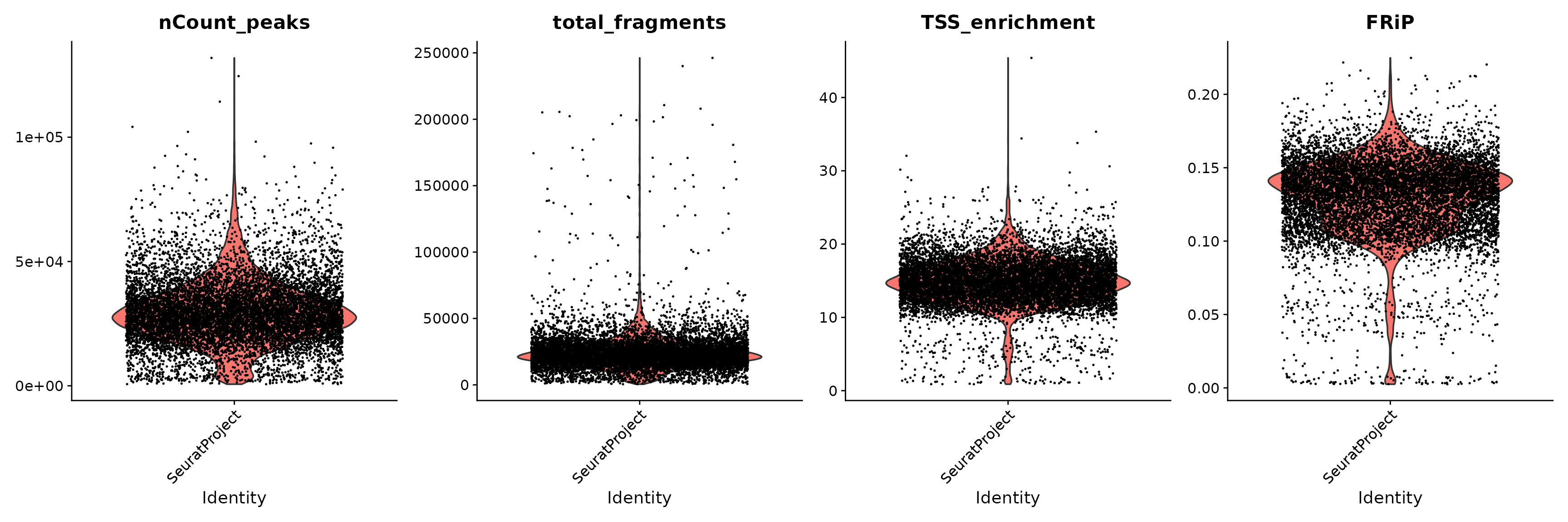
We can plot the distribution of each QC metric separately using a violin plot:
VlnPlot(
  object = pbmc,
  features = c("nCount_peaks", "total_fragments", "TSS_enrichment", "FRiP"),
  pt.size = 0.1,
  ncol = 4
)
Finally we remove cells that are outliers for these QC metrics. The exact QC thresholds used will need to be adjusted according to your dataset.
pbmc <- subset(
  x = pbmc,
  subset = total_fragments > 10000 &
    total_fragments < 90000 &
    TSS_enrichment > 10 &
    FRiP > 0.1
)
pbmc
## An object of class Seurat
## 165376 features across 8828 samples within 1 assay
## Active assay: peaks (165376 features, 0 variable features)
## 1 layer present: countsNormalization and linear dimensional reduction
Normalization: Signac performs term frequency-inverse document frequency (TF-IDF) normalization. This is a two-step normalization procedure, that both normalizes across cells to correct for differences in cellular sequencing depth, and across peaks to give higher values to more rare peaks.
Feature selection: The low dynamic range of scATAC-seq data makes it challenging to perform variable feature selection, as we do for scRNA-seq. Instead, we can choose to use only the top n% of features (peaks) for dimensional reduction, or remove features present in less than n cells with the
FindTopFeatures()function. Here we will use all features, though we have seen very similar results when using only a subset of features (try setting min.cutoff to ‘q75’ to use the top 25% all peaks), with faster runtimes. Features used for dimensional reduction are automatically set asVariableFeatures()for the Seurat object by this function.Dimension reduction: We next run singular value decomposition (SVD) on the TD-IDF matrix, using the features (peaks) selected above. This returns a reduced dimension representation of the object (for users who are more familiar with scRNA-seq, you can think of this as analogous to the output of PCA).
The combined steps of TF-IDF followed by SVD are known as latent semantic indexing (LSI), and were first introduced for the analysis of scATAC-seq data by Cusanovich et al. 2015.
pbmc <- RunTFIDF(pbmc)
pbmc <- FindTopFeatures(pbmc, min.cutoff = "q0")
pbmc <- RunSVD(pbmc)
The first LSI component often captures sequencing depth (technical
variation) rather than biological variation. If this is the case, the
component should be removed from downstream analysis. We can assess the
correlation between each LSI component and sequencing depth using the
DepthCor() function:
DepthCor(pbmc)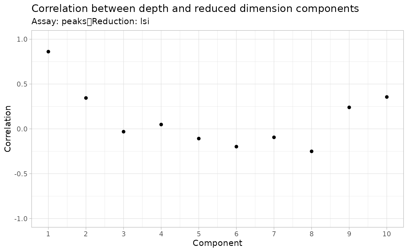
Here we see there is a very strong correlation between the first LSI component and the total number of counts for the cell. We will perform downstream steps without this component as we don’t want to group cells together based on their total sequencing depth, but rather by their patterns of accessibility at cell-type-specific peaks.
Non-linear dimension reduction and clustering
Now that the cells are embedded in a low-dimensional space we can use
methods commonly applied for the analysis of scRNA-seq data to perform
graph-based clustering and non-linear dimension reduction for
visualization. The functions RunUMAP(),
FindNeighbors(), and FindClusters() all come
from the Seurat package.
pbmc <- RunUMAP(object = pbmc, reduction = "lsi", dims = 2:30)
pbmc <- FindNeighbors(object = pbmc, reduction = "lsi", dims = 2:30)
pbmc <- FindClusters(object = pbmc, verbose = FALSE, algorithm = 3)
DimPlot(object = pbmc, label = TRUE) + NoLegend()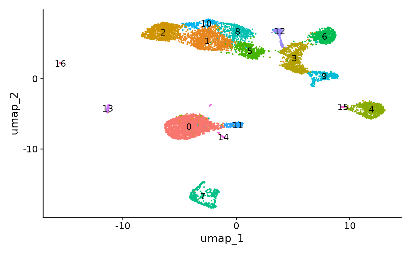
Create a gene activity matrix
The UMAP visualization reveals the presence of multiple cell groups in human blood. If you are familiar with scRNA-seq analyses of PBMC, you may recognize the presence of certain myeloid and lymphoid populations in the scATAC-seq data. However, annotating and interpreting clusters is more challenging in scATAC-seq data as much less is known about the functional roles of noncoding genomic regions than is known about protein coding regions (genes).
We can try to quantify the activity of each gene in the genome by assessing the chromatin accessibility associated with the gene, and create a new gene activity assay derived from the scATAC-seq data. Here we will use a simple approach of summing the fragments intersecting the gene body and promoter region (we also recommend exploring the Cicero tool, which can accomplish a similar goal, and we provide a vignette showing how to run Cicero within a Signac workflow here).
To create a gene activity matrix, we extract gene coordinates and
extend them to include the 2 kb upstream region (as promoter
accessibility is often correlated with gene expression). We then count
the number of fragments for each cell that map to each of these regions,
using the using the FeatureMatrix() function. These steps
are automatically performed by the GeneActivity()
function:
gene.activities <- GeneActivity(pbmc)
# add the gene activity matrix to the Seurat object as a new assay and normalize it
pbmc[["RNA"]] <- CreateAssayObject(counts = gene.activities)
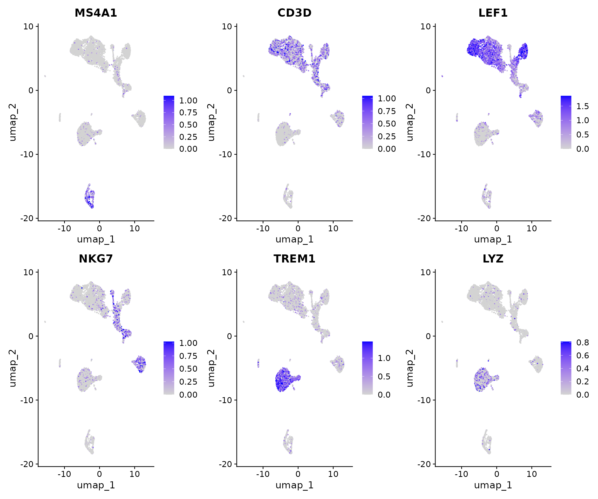
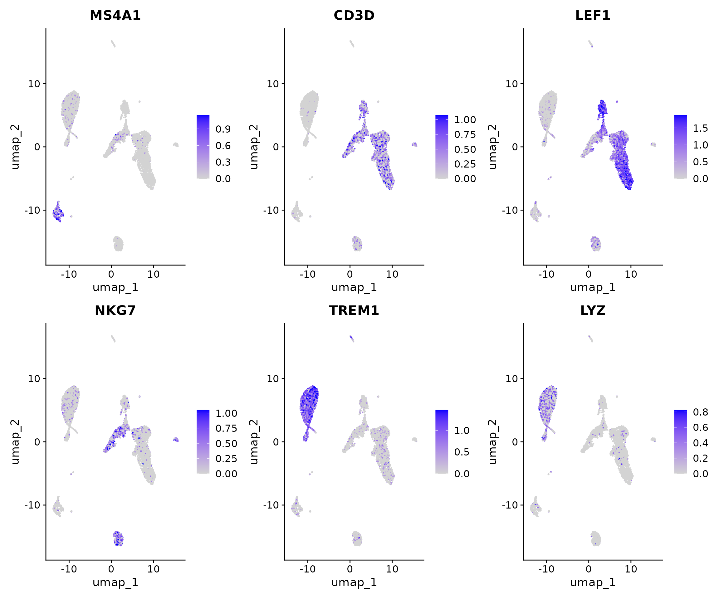
pbmc <- NormalizeData(pbmc, assay = "RNA")Now we can visualize the activities of canonical marker genes to help interpret our ATAC-seq clusters. Note that the activities will be much noisier than scRNA-seq measurements. This is because they represent measurements from sparse chromatin data, and because they assume a general correspondence between gene body/promoter accessibility and gene expression which may not always be the case. Nonetheless, we can begin to discern populations of monocytes, B, T, and NK cells based on these gene activity profiles. However, further subdivision of these cell types is challenging based on supervised analysis alone.
DefaultAssay(pbmc) <- "RNA"

FeaturePlot(
  object = pbmc,
  features = c("MS4A1", "CD3D", "LEF1", "NKG7", "TREM1", "LYZ"),
  pt.size = 0.1,
  max.cutoff = "q95",
  ncol = 3
)
Integrating with scRNA-seq data
To help interpret the scATAC-seq data, we can classify cells based on an scRNA-seq experiment from the same biological system (human PBMC). We utilize methods for cross-modality integration and label transfer, described here, with a more in-depth tutorial here. We aim to identify shared correlation patterns in the gene activity matrix and scRNA-seq dataset to identify matched biological states across the two modalities. This procedure returns a classification score for each cell for each scRNA-seq-defined cluster label.
Here we load a pre-processed scRNA-seq dataset for human PBMCs, also provided by 10x Genomics. You can download the raw data for this experiment from the 10x website, and view the code used to construct this object on GitHub. Alternatively, you can download the pre-processed Seurat object here.
# Load the pre-processed scRNA-seq data for PBMCs
pbmc_rna <- readRDS("pbmc_10k_v3.rds")
pbmc_rna <- UpdateSeuratObject(pbmc_rna)
transfer.anchors <- FindTransferAnchors(
  reference = pbmc_rna,
  query = pbmc,
  reduction = "cca"
)
## Running CCA## Merging objects## Finding neighborhoods## Finding anchors## Found 18284 anchors
predicted.labels <- TransferData(
  anchorset = transfer.anchors,
  refdata = pbmc_rna$celltype,
  weight.reduction = pbmc[["lsi"]],
  dims = 2:30
)
## Finding integration vectors## Finding integration vector weights## Predicting cell labels
pbmc <- AddMetaData(object = pbmc, metadata = predicted.labels)
plot1 <- DimPlot(
  object = pbmc_rna,
  group.by = "celltype",
  label = TRUE,
  repel = TRUE
) + NoLegend() + ggtitle("scRNA-seq")

plot2 <- DimPlot(
  object = pbmc,
  group.by = "predicted.id",
  label = TRUE,
  repel = TRUE
) + NoLegend() + ggtitle("scATAC-seq")

plot1 + plot2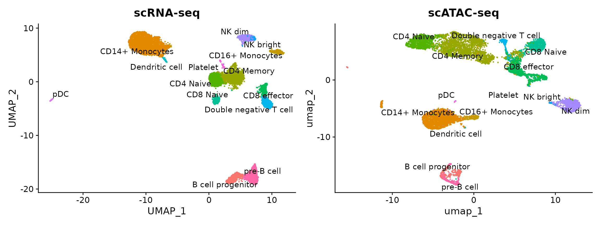
You can see that the scRNA-based classifications are consistent with the UMAP visualization that was computed using the scATAC-seq data. Notice, however, that a small population of cells are predicted to be platelets in the scATAC-seq dataset. This is unexpected as platelets are not nucleated and should not be detected by scATAC-seq. It is possible that the cells predicted to be platelets could instead be the platelet-precursors megakaryocytes, which largely reside in the bone marrow but are rarely found in the peripheral blood of healthy patients, such as the individual these PBMCs were drawn from. Given the already extreme rarity of megakaryocytes within normal bone marrow (< 0.1%), this scenario seems unlikely.
A closer look at the “platelets”
Plotting the prediction score for the cells assigned to each label reveals that the “platelet” cells received relatively low scores (< 0.8), indicating a low confidence in the assigned cell identity. In most cases, the next most likely cell identity predicted for these cells was “CD4 naive”.
VlnPlot(pbmc, "prediction.score.max", group.by = "predicted.id")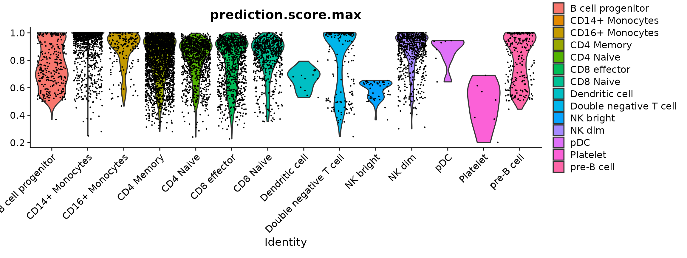
# Identify the metadata columns that start with "prediction.score."
metadata_attributes <- colnames(pbmc[[]])
prediction_score_attributes <- grep("^prediction.score.", metadata_attributes, value = TRUE)
prediction_score_attributes <- setdiff(prediction_score_attributes, "prediction.score.max")

# Extract the prediction score attributes for these cells
predicted_platelets <- which(pbmc$predicted.id == "Platelet")
platelet_scores <- pbmc[[]][predicted_platelets, prediction_score_attributes]

# Order the columns by their average values in descending order
ordered_columns <- names(sort(colMeans(platelet_scores, na.rm = TRUE), decreasing = TRUE))
ordered_platelet_scores_df <- platelet_scores[, ordered_columns]

print(ordered_platelet_scores_df)
## prediction.score.Platelet prediction.score.CD4.Memory prediction.score.CD8.Naive prediction.score.pDC prediction.score.CD14..Monocytes prediction.score.CD4.Naive prediction.score.CD8.effector prediction.score.NK.dim prediction.score.NK.bright prediction.score.pre.B.cell prediction.score.Double.negative.T.cell prediction.score.Dendritic.cell prediction.score.CD16..Monocytes prediction.score.B.cell.progenitor
## AACAGTCTCTTCCGTG-1 0.3838710 0.212994418 0.272006697 0.00000000 0.003359445 0.03754429 0.072812740 0.0000000000 0.00000000 0.003280782 0.01413066 0.000000000 0 0
## AGCGTGCGTCAGACGA-1 0.2027993 0.169663081 0.020306831 0.00000000 0.000000000 0.08720040 0.096287064 0.1993467743 0.18180994 0.015542124 0.02704445 0.000000000 0 0
## CACTAAGGTAATGTAG-1 0.5719986 0.000000000 0.031246562 0.23745349 0.024351820 0.08079918 0.000000000 0.0008924242 0.00000000 0.053257936 0.00000000 0.000000000 0 0
## CTCAACCAGCGAGCTA-1 0.6903416 0.003653886 0.007154750 0.09270494 0.127028120 0.04062775 0.002906345 0.0000000000 0.00000000 0.026558113 0.00000000 0.009024522 0 0
## GCCTACTGTTCTTTGT-1 0.3718940 0.247085454 0.030461298 0.00000000 0.000000000 0.06841244 0.154628712 0.0337916986 0.04241446 0.000000000 0.05131198 0.000000000 0 0
## GCTTAAGCAAAGGTCG-1 0.6155275 0.002539134 0.006909659 0.07191388 0.200808101 0.05956563 0.004155151 0.0000000000 0.00000000 0.026018043 0.00000000 0.012562868 0 0
## TCCAGAAGTAGCGTTT-1 0.5109697 0.365251705 0.059396745 0.00000000 0.031092307 0.00000000 0.009412582 0.0000000000 0.00000000 0.000000000 0.02387695 0.000000000 0 0As there are only a very small number of cells classified as “platelets” (< 20), it is difficult to figure out their precise cellular identity. Larger datasets would be required to confidently identify specific peaks for this population of cells, and further analysis performed to correctly annotate them. For downstream analysis we will thus remove the extremely rare cell states that were predicted, retaining only cell annotations with >20 cells total.
predicted_id_counts <- table(pbmc$predicted.id)

# Identify the predicted.id values that have more than 20 cells
major_predicted_ids <- names(predicted_id_counts[predicted_id_counts > 20])
pbmc <- pbmc[, pbmc$predicted.id %in% major_predicted_ids]
For downstream analyses, we can simply reassign the identities of each cell from their UMAP cluster index to the per-cell predicted labels. It is also possible to consider merging the cluster indexes and predicted labels.
# change cell identities to the per-cell predicted labels
Idents(pbmc) <- pbmc$predicted.id
To combine clustering and label transfer results
Alternatively, in instances where we wish to combine our scATAC-seq clustering and label transfer results, we can reassign the identities of all cells within each UMAP cluster to the most common predicted label for that cluster.
Find differentially accessible peaks between cell types
To find differentially accessible regions between clusters of cells, we can perform a differential accessibility (DA) test. A simple approach is to perform a Wilcoxon rank sum test, and the presto package has implemented an extremely fast Wilcoxon test that can be run on a Seurat object.
Install presto
if (!requireNamespace("remotes", quietly = TRUE)) {
  install.packages("remotes")
}
remotes::install_github("immunogenomics/presto")
Here we will focus on comparing Naive CD4 cells and CD14 monocytes, but any groups of cells can be compared using these methods. We can also visualize these marker peaks on a violin plot, feature plot, dot plot, heat map, or any visualization tool in Seurat.
# change back to working with peaks instead of gene activities
DefaultAssay(pbmc) <- "peaks"

# wilcox is the default option for test.use
da_peaks <- FindMarkers(
  object = pbmc,
  ident.1 = "CD4 Naive",
  ident.2 = "CD14+ Monocytes",
  test.use = "wilcox",
  min.pct = 0.1
)

head(da_peaks)
## p_val avg_log2FC pct.1 pct.2 p_val_adj
## chr12:119988511-119989430 0.000000e+00 4.052999 0.796 0.096 0.000000e+00
## chr7:142808530-142809435 0.000000e+00 3.655951 0.768 0.093 0.000000e+00
## chr17:82126458-82127377 0.000000e+00 4.829170 0.718 0.048 0.000000e+00
## chr7:138752283-138753197 0.000000e+00 4.769039 0.701 0.051 0.000000e+00
## chr4:152100248-152101142 9.754486e-315 4.967818 0.638 0.038 1.613158e-309
## chr11:60985909-60986801 3.677048e-308 4.400857 0.666 0.067 6.080954e-303Logistic regression with total fragment number as the latent variable
Another approach for differential testing is to utilize logistic regression for, as suggested by Ntranos et al. 2018 for scRNA-seq data, and add the total number of fragments as a latent variable to mitigate the effect of differential sequencing depth on the result.
# change back to working with peaks instead of gene activities
DefaultAssay(pbmc) <- "peaks"

# Use logistic regression, set total fragment no. as latent var
lr_da_peaks <- FindMarkers(
  object = pbmc,
  ident.1 = "CD4 Naive",
  ident.2 = "CD14+ Monocytes",
  test.use = "LR",
  latent.vars = "nCount_peaks",
  min.pct = 0.1
)
head(lr_da_peaks)
plot1 <- VlnPlot(
  object = pbmc,
  features = rownames(da_peaks)[1],
  pt.size = 0.1,
  idents = c("CD4 Naive", "CD14+ Monocytes")
)
plot2 <- FeaturePlot(
  object = pbmc,
  features = rownames(da_peaks)[1],
  pt.size = 0.1
)

plot1 | plot2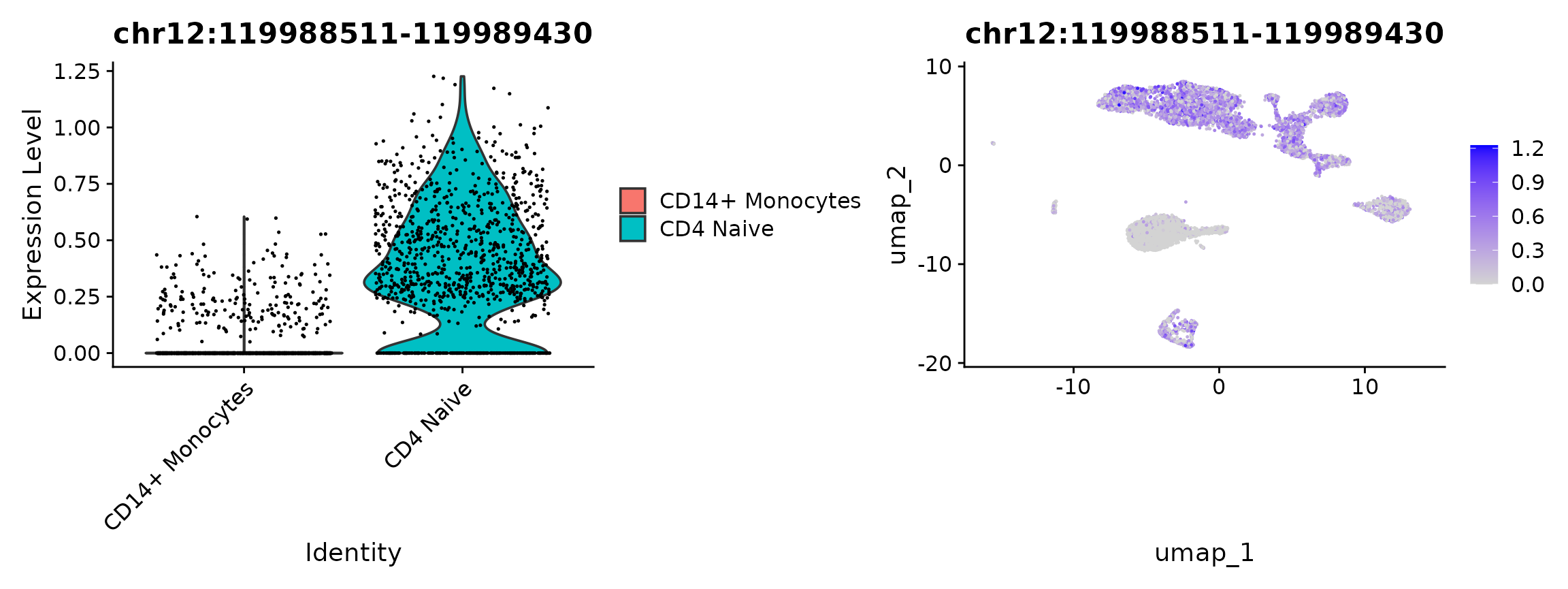
Peak coordinates can be difficult to interpret alone. We can find the
closest gene to each of these peaks using functions from the
GenomicRanges package:
open_cd4naive <- rownames(da_peaks[da_peaks$avg_log2FC > 3, ])

gene_distance_cd4naive <- distanceToNearest(GRanges(open_cd4naive), Annotation(pbmc))

closest_genes <- data.frame(
  peak = open_cd4naive,
  gene_name = Annotation(pbmc)[subjectHits(gene_distance_cd4naive)]$gene_name,
  gene_id = Annotation(pbmc)[subjectHits(gene_distance_cd4naive)]$gene_id,
  distance = mcols(gene_distance_cd4naive)$distance
)
head(closest_genes)## peak gene_name gene_id distance
## 1 chr12:119988511-119989430 BICDL1 ENSG00000135127 438
## 2 chr7:142808530-142809435 PRSS2 ENSG00000275896 33965
## 3 chr17:82126458-82127377 CCDC57 ENSG00000176155 0
## 4 chr7:138752283-138753197 ATP6V0A4 ENSG00000105929 0
## 5 chr4:152100248-152101142 FBXW7 ENSG00000109670 219401
## 6 chr11:60985909-60986801 CD6 ENSG00000013725 0We could follow up with this result by doing gene ontology enrichment
analysis on the gene sets close to differentially accessible peaks, and
there are many R packages that can do this (see the GOstats
or clusterProfiler
packages for example).
GO enrichment analysis with clusterProfiler
library(clusterProfiler)
library(org.Hs.eg.db)
library(enrichplot)
cd4naive_ego <- enrichGO(
  gene = closest_genes$gene_id,
  keyType = "ENSEMBL",
  OrgDb = org.Hs.eg.db,
  ont = "BP",
  pAdjustMethod = "BH",
  pvalueCutoff = 0.05,
  qvalueCutoff = 0.05,
  readable = TRUE
)

barplot(cd4naive_ego, showCategory = 20)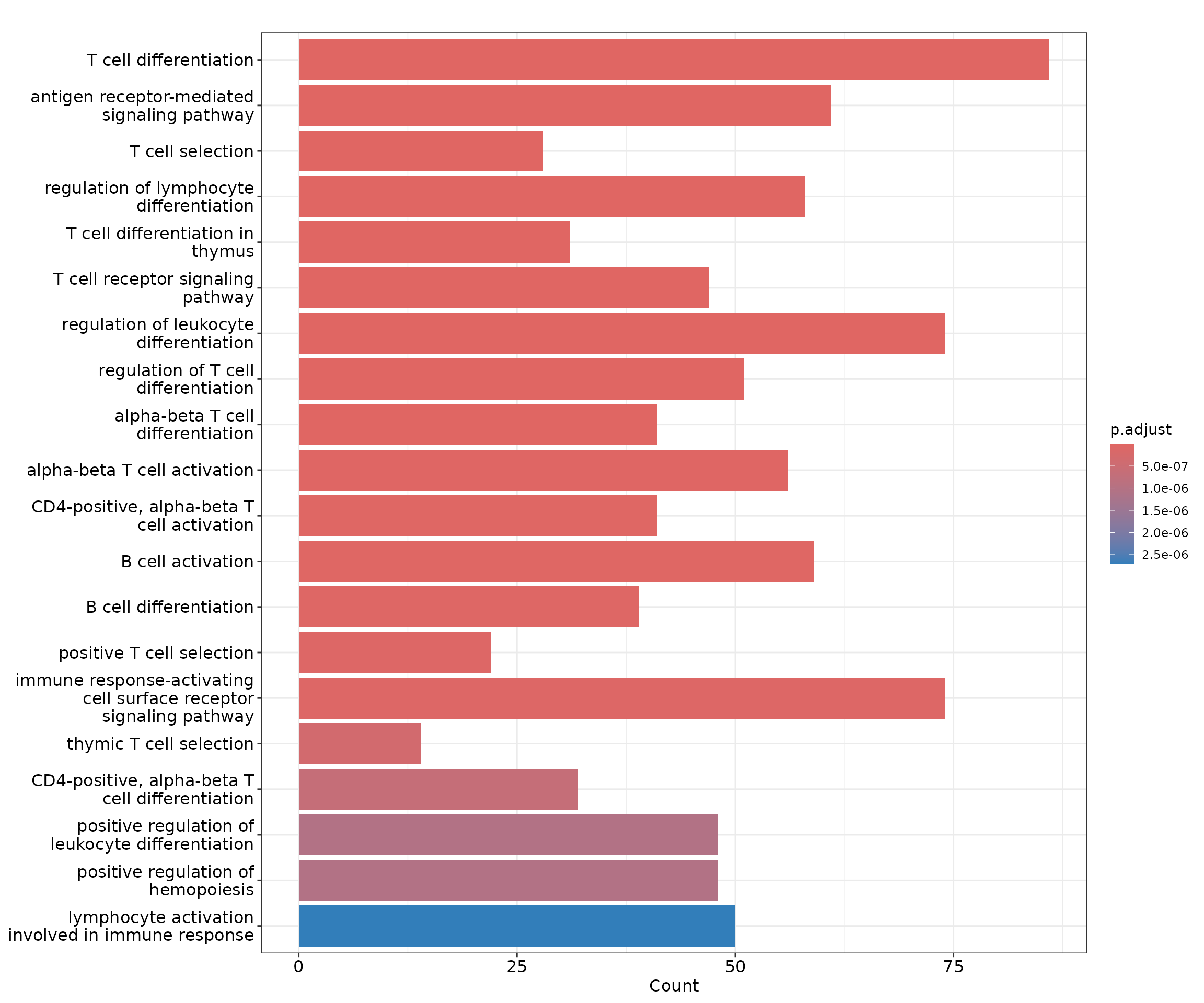
Alternatively, we can find marker peaks for all cell types using the
FindAllMarkers function and visualize them in one plot using
MultiCoveragePlot().
# find marker peaks for all clusters
markers <- FindAllMarkers(object = pbmc)
## Calculating cluster CD14+ Monocytes## Calculating cluster B cell progenitor## Calculating cluster CD4 Memory## Calculating cluster NK dim## Calculating cluster CD8 Naive## Calculating cluster pre-B cell## Calculating cluster CD8 effector## Calculating cluster CD4 Naive## Calculating cluster Double negative T cell## Calculating cluster NK bright## Calculating cluster CD16+ Monocytes
# sort and select top marker peak for each cell cluster
markers_sorted <- markers |>
  group_by(cluster) |>
  arrange(desc(avg_log2FC), desc(pct.1), .by_group = TRUE) |>
  slice_head(n = 1)
MultiCoveragePlot(
  object = pbmc,
  regions = markers_sorted$gene,
  extend.upstream = 500,
  extend.downstream = 500
)
Plotting genomic regions
We can plot the frequency of Tn5 integration across regions of the
genome for cells grouped by cluster, cell type, or any other metadata
stored in the object for any genomic region using the
CoveragePlot() function. These represent pseudo-bulk
accessibility tracks, where signal from all cells within a group have
been averaged together to visualize the DNA accessibility in a region
(thanks to Andrew Hill for giving the inspiration for this function in
his excellent blog
post). Alongside these accessibility tracks we can visualize other
important information including gene annotation, peak coordinates, and
genomic links (if they’re stored in the object). See the visualization vignette for more
information.
For plotting purposes, it’s nice to have related cell types grouped
together. We can automatically sort the plotting order according to
similarities across the annotated cell types by running the
SortIdents() function:
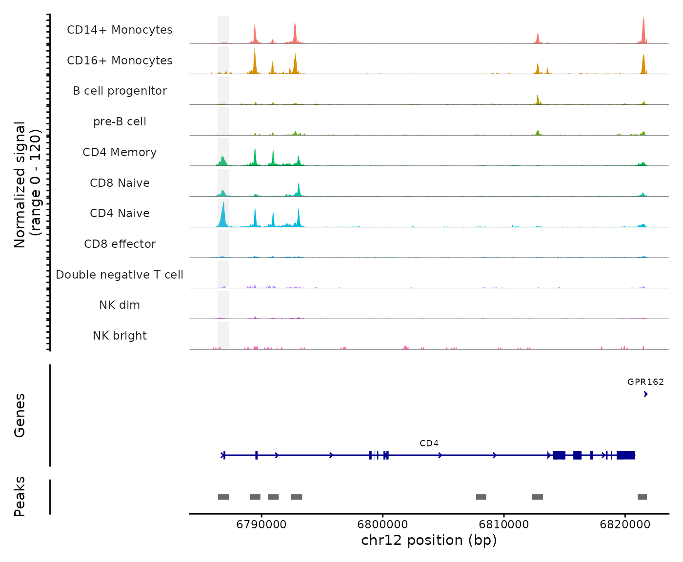
pbmc <- SortIdents(pbmc)We can then visualize the DA peaks open in CD4 naive cells and CD14 monocytes, near some key marker genes for these cell types, CD4 and LYZ respectively. Here we’ll highlight the DA peaks regions in grey.
# find DA peaks overlapping gene of interest
regions_highlight <- subsetByOverlaps(GRanges(open_cd4naive), LookupGeneCoords(pbmc, "CD4"))

CoveragePlot(
  object = pbmc,
  region = "CD4",
  region.highlight = regions_highlight,
  extend.upstream = 1000,
  extend.downstream = 1000
)
Working with datasets that were not quantified using CellRanger
The CellRanger software from 10x Genomics generates several useful QC metrics per-cell, as well as a peak/cell matrix and an indexed fragments file. In the above vignette, we utilize the CellRanger outputs, but provide alternative functions in Signac for many of the same purposes here.
Generating a peak/cell or bin/cell matrix
The FeatureMatrix function can be used to generate a
count matrix containing any set of genomic ranges in its rows. These
regions could be a set of peaks, or bins that span the entire
genome.
# not run
# peak_ranges should be a set of genomic ranges spanning the set of peaks to be quantified per cell
peak_matrix <- FeatureMatrix(
  fragments = Fragments(pbmc),
  features = peak_ranges
)
For convenience, we also include a GenomeBinMatrix()
function that will generate a set of genomic ranges spanning the entire
genome for you, and run FeatureMatrix() internally to
produce a genome bin/cell matrix.
# not run
library(BSgenome.Hsapiens.UCSC.hg38)
bin_matrix <- GenomeBinMatrix(
  fragments = Fragments(pbmc),
  genome = seqlengths(BSgenome.Hsapiens.UCSC.hg38),
  binsize = 5000
)
This tab demonstrates an alternative workflow using regulatory element modules (REMO) rather than de novo peak calling. By using REMO, we can skip the peak calling step and ensure that our dataset can be easily compared to other datasets. We can also use REMO to perform some automated cell annotation, demonstrated at the end of this tab.
REMO can be installed from GitHub:
remotes::install_github("stuart-lab/REMO.v1.GRCh38")Pre-processing workflow
First load Signac, Seurat, and some other packages we will be using for analyzing human data.
library(Signac)
library(Seurat)
library(GenomicRanges)
library(ggplot2)
library(patchwork)
library(GenomeInfoDb)
library(REMO.v1.GRCh38)
Defining gene annotations
Multiple gene annotation patches are released for each genome assembly. It is advisable to always use the annotations from the same assembly patch that was used to perform the read mapping.
From the dataset summary, we can see that the reference package 10x Genomics used to perform the mapping was “GRCh38-2020-A”, which corresponds to the Ensembl v98 patch release. For more information on the various Ensembl releases, you can refer to this site.
# load gene annotations
library(AnnotationHub)
ah <- AnnotationHub()

ensdb_v98 <- ah[["AH75011"]]
annotations <- GetGRangesFromEnsDb(ensdb = ensdb_v98)

# change to UCSC style since the data was mapped to hg38
seqlevelsStyle(annotations) <- "UCSC"
Quality control metrics
We can compute quality control metrics for the scATAC-seq data using
the ATACqc function. These metrics include:
Nucleosome banding pattern: The histogram of DNA fragment sizes (determined from the paired-end sequencing reads) should exhibit a strong nucleosome banding pattern corresponding to the length of DNA wrapped around a single nucleosome. We calculate this per single cell, and quantify the approximate ratio of mononucleosomal to nucleosome-free fragments (stored as
Nucleosome_signal)Transcriptional start site (TSS) enrichment score: The ENCODE project has defined an ATAC-seq targeting score based on the ratio of fragments centered at the TSS to fragments in TSS-flanking regions (see https://www.encodeproject.org/data-standards/terms/). Poor ATAC-seq experiments typically will have a low TSS enrichment score. Results are stored in metadata under the column name
TSS_enrichment.Total number of fragments: A measure of cellular sequencing depth / complexity. Cells with very few fragments may need to be excluded due to low sequencing depth. Cells with extremely high levels may represent doublets, nuclei clumps, or other artefacts. This is stored as
total_fragments
Here we run ATACqc() directly on the fragment file to
efficiently compute these QC metrics for every observed cell
barcode:
frags <- "10k_pbmc_ATACv2_nextgem_Chromium_Controller_fragments.tsv.gz"
metadata <- ATACqc(object = frags, annotations = annotations)
head(metadata)
## TSS_flank TSS_center total_fragments TSS_enrichment FRiP Nucleosome_signal Mito_fragments Mito_fraction chrX_fragments chrX_fraction chrY_fragments chrY_fraction
## CAACGTACACTACACA-1 0 0 1 0 0.0000 0.0000 0 0 0 0.0000 0 0
## ACCGCAGGTATTCGCA-1 0 0 3 0 0.0000 1.0000 0 0 0 0.0000 0 0
## AGCTGTAGTCATCGTA-1 0 9 95 0 0.0947 0.5577 0 0 5 0.0526 0 0
## CTAGGGCCACCATTCC-1 0 0 1 0 0.0000 0.0000 0 0 0 0.0000 0 0
## TTGGTCCGTAGTATCC-1 0 0 1 0 0.0000 0.0000 0 0 1 1.0000 0 0
## TTACGGACACTCAAGT-1 1 7 99 7 0.0707 1.1951 0 0 1 0.0101 0 0Matrix quantification
We can start by selecting cells to include in the matrix quantification by setting some permissive QC thresholds:
cells <- rownames(metadata[metadata$TSS_enrichment > 5 & metadata$total_fragments > 8000, ])This gives us an initial set of cell barcodes to work with, that we can include in the matrix quantification step. Here we will create a REMO matrix using fragtk:
remo <- RunFragtk(
  fragments = frags,
  features = REMO.v1.GRCh38,
  cells = cells,
  group = TRUE
)
## Grouping regions by column: REMO## Loading count matrix
dim(remo)## [1] 340069 9693Constructing the Seurat object
Next we can create a Seurat object containing a
ChromatinAssay5-class assay object storing the chromatin
accessibility data.
chrom_assay <- CreateChromatinAssay5(
  counts = remo,
  fragments = frags,
  annotation = annotations,
  min.cells = 20
)
## Computing hash
pbmc <- CreateSeuratObject(
  counts = chrom_assay,
  assay = "REMO",
  meta.data = metadata,
  min.cells = 20
)
pbmc## An object of class Seurat
## 203933 features across 9693 samples within 1 assay
## Active assay: REMO (203933 features, 0 variable features)
## 1 layer present: countsQuality control filtering
Next we can perform some more stringent QC filtering on the object:
VlnPlot(
  object = pbmc,
  features = c("TSS_enrichment", "Nucleosome_signal", "total_fragments"),
  group.by = "orig.ident",
  ncol = 3,
  pt.size = 0
)
## Warning: Default search for "data" layer in "REMO" assay yielded no results; utilizing "counts" layer instead.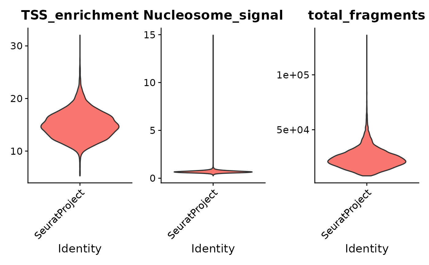
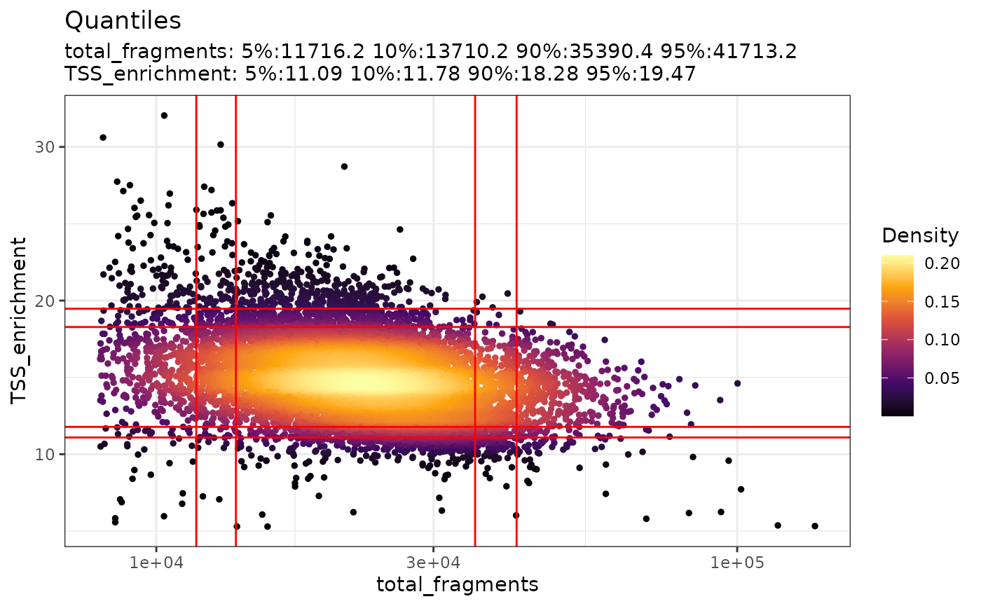
The relationship between variables stored in the object metadata can
be visualized using the DensityScatter() function. This can
also be used to quickly find suitable cutoff values for different QC
metrics by setting quantiles=TRUE:
DensityScatter(
  object = pbmc,
  x = "total_fragments",
  y = "TSS_enrichment",
  log_x = TRUE,
  quantiles = TRUE
)
Doublet removal (optional)
We can predict doublets using the scDblFinder
package:
library(scDblFinder)

# doublet score
scDbl <- as.SingleCellExperiment(pbmc)
scDbl <- scDblFinder(scDbl)

pbmc$dbl.class <- scDbl$scDblFinder.class
pbmc$dbl.score <- scDbl$scDblFinder.score
pbmc <- subset(pbmc, total_fragments > 10000 &
  total_fragments < 60000 &
  TSS_enrichment > 9 &
  dbl.class == "singlet")
pbmc## An object of class Seurat
## 203933 features across 8457 samples within 1 assay
## Active assay: REMO (203933 features, 0 variable features)
## 1 layer present: countsFeature selection
We can select highly variable REMO modules by modelling the
mean-variance relationship. Here we use the FitMeanVar()
function in Signac, which will fit a loess curve to the log(mean) and
log(variance) of each feature, and then estimate the residual variance
for each feature given the mean. This is similar to how the
FindVariableFeatures() function in Seurat works, but is
more efficient for a large number of features as we downsample the
features when fitting the loess model.
pbmc <- FitMeanVar(pbmc)## Finding variable features for layer counts## Retained 203933 features after count filteringNormalization and linear dimensional reduction
Next we perform data normalization and dimension reduction. Here we
use the RunSVD() function with pca=TRUE to
efficiently compute PCA without storing the full standardized data
matrix in memory:
pbmc <- NormalizeData(pbmc)## Normalizing layer: counts
pbmc <- RunSVD(pbmc, pca = TRUE)## Running PCANon-linear dimension reduction and clustering
Now that the cells are embedded in a low-dimensional space we can use
methods commonly applied for the analysis of scRNA-seq data to perform
graph-based clustering and non-linear dimension reduction for
visualization. The functions RunUMAP(),
FindNeighbors(), and FindClusters() all come
from the Seurat package.
pbmc <- RunUMAP(object = pbmc, dims = 1:40)
pbmc <- FindNeighbors(object = pbmc, dims = 1:40)
pbmc <- FindClusters(object = pbmc, verbose = FALSE, algorithm = 3)
DimPlot(object = pbmc, label = TRUE) + NoLegend()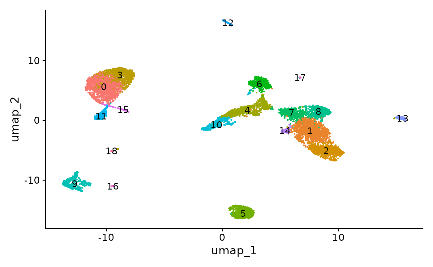
Create a gene activity matrix
The UMAP visualization reveals the presence of multiple cell groups in human blood. If you are familiar with scRNA-seq analyses of PBMC, you may recognize the presence of certain myeloid and lymphoid populations in the scATAC-seq data. However, annotating and interpreting clusters is more challenging in scATAC-seq data as much less is known about the functional roles of noncoding genomic regions than is known about protein coding regions (genes).
We can try to quantify the activity of each gene in the genome by assessing the chromatin accessibility associated with the gene, and create a new gene activity assay derived from the scATAC-seq data. Here we will use a simple approach of summing the fragments intersecting the gene body and promoter region (we also recommend exploring the Cicero tool, which can accomplish a similar goal, and we provide a vignette showing how to run Cicero within a Signac workflow here).
To create a gene activity matrix, we extract gene coordinates and
extend them to include the 2 kb upstream region (as promoter
accessibility is often correlated with gene expression). We then count
the number of fragments for each cell that map to each of these regions,
using the using the FeatureMatrix() function. These steps
are automatically performed by the GeneActivity()
function:
gene.activities <- GeneActivity(pbmc)
# add the gene activity matrix to the Seurat object as a new assay and normalize it
pbmc[["RNA"]] <- CreateAssay5Object(counts = gene.activities)
pbmc <- NormalizeData(pbmc, assay = "RNA")
Now we can visualize the activities of canonical marker genes to help interpret our ATAC-seq clusters. Note that the activities will be much noisier than scRNA-seq measurements. This is because they represent measurements from sparse chromatin data, and because they assume a general correspondence between gene body/promoter accessibility and gene expression which may not always be the case. Nonetheless, we can begin to discern populations of monocytes, B, T, and NK cells based on these gene activity profiles. However, further subdivision of these cell types is challenging based on supervised analysis alone.
DefaultAssay(pbmc) <- "RNA"

FeaturePlot(
  object = pbmc,
  features = c("MS4A1", "CD3D", "LEF1", "NKG7", "TREM1", "LYZ"),
  pt.size = 0.1,
  max.cutoff = "q95",
  ncol = 3
)
Integrating with scRNA-seq data
To help interpret the scATAC-seq data, we can classify cells based on an scRNA-seq experiment from the same biological system (human PBMC). We utilize methods for cross-modality integration and label transfer, described here, with a more in-depth tutorial here. We aim to identify shared correlation patterns in the gene activity matrix and scRNA-seq dataset to identify matched biological states across the two modalities. This procedure returns a classification score for each cell for each scRNA-seq-defined cluster label.
Here we load a pre-processed scRNA-seq dataset for human PBMCs, also provided by 10x Genomics. You can download the raw data for this experiment from the 10x website, and view the code used to construct this object on GitHub. Alternatively, you can download the pre-processed Seurat object here.
# Load the pre-processed scRNA-seq data for PBMCs
pbmc_rna <- readRDS("pbmc_10k_v3.rds")
pbmc_rna <- UpdateSeuratObject(pbmc_rna)
transfer.anchors <- FindTransferAnchors(
  reference = pbmc_rna,
  query = pbmc,
  reduction = "cca"
)
## Running CCA## Merging objects## Finding neighborhoods## Finding anchors## Found 18219 anchors
predicted.labels <- TransferData(
  anchorset = transfer.anchors,
  refdata = pbmc_rna$celltype,
  weight.reduction = pbmc[["pca"]],
  dims = 1:30
)
## Finding integration vectors## Finding integration vector weights## Predicting cell labels
pbmc <- AddMetaData(object = pbmc, metadata = predicted.labels)
plot1 <- DimPlot(
  object = pbmc_rna,
  group.by = "celltype",
  label = TRUE,
  repel = TRUE
) + NoLegend() + ggtitle("scRNA-seq")

plot2 <- DimPlot(
  object = pbmc,
  group.by = "predicted.id",
  label = TRUE,
  repel = TRUE
) + NoLegend() + ggtitle("scATAC-seq")

plot1 + plot2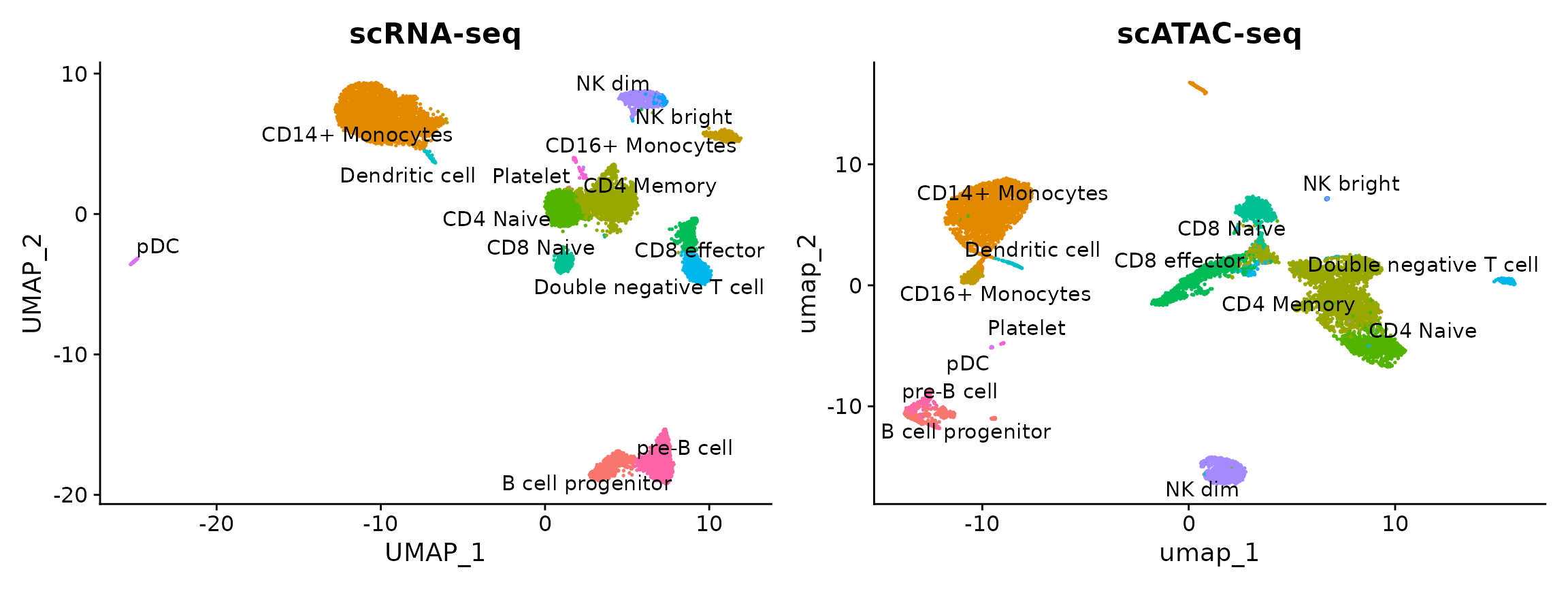
You can see that the scRNA-based classifications are consistent with the UMAP visualization that was computed using the scATAC-seq data. Notice, however, that a small population of cells are predicted to be platelets in the scATAC-seq dataset. This is unexpected as platelets are not nucleated and should not be detected by scATAC-seq. It is possible that the cells predicted to be platelets could instead be the platelet-precursors megakaryocytes, which largely reside in the bone marrow but are rarely found in the peripheral blood of healthy patients, such as the individual these PBMCs were drawn from. Given the already extreme rarity of megakaryocytes within normal bone marrow (< 0.1%), this scenario seems unlikely.
A closer look at the “platelets”
Plotting the prediction score for the cells assigned to each label reveals that the “platelet” cells received relatively low scores (< 0.8), indicating a low confidence in the assigned cell identity. In most cases, the next most likely cell identity predicted for these cells was “CD4 naive”.
VlnPlot(pbmc, "prediction.score.max", group.by = "predicted.id")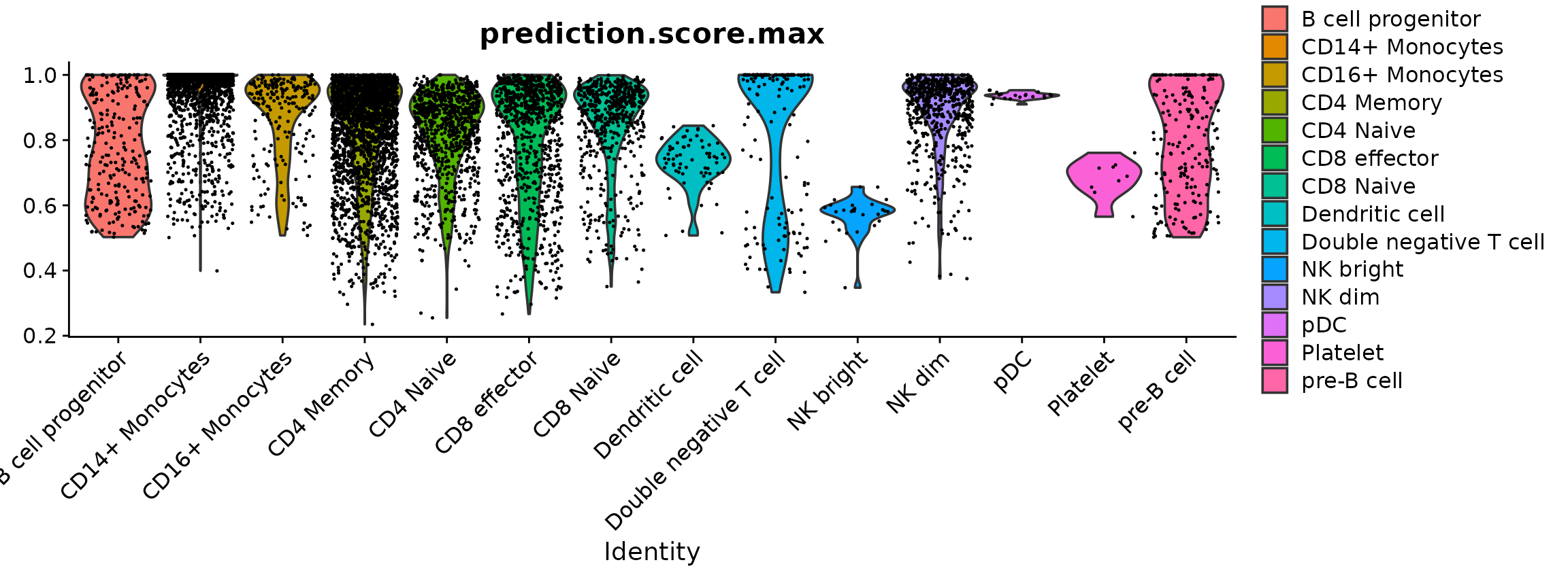
# Identify the metadata columns that start with "prediction.score."
metadata_attributes <- colnames(pbmc[[]])
prediction_score_attributes <- grep("^prediction.score.", metadata_attributes, value = TRUE)
prediction_score_attributes <- setdiff(prediction_score_attributes, "prediction.score.max")

# Extract the prediction score attributes for these cells
predicted_platelets <- which(pbmc$predicted.id == "Platelet")
platelet_scores <- pbmc[[]][predicted_platelets, prediction_score_attributes]

# Order the columns by their average values in descending order
ordered_columns <- names(sort(colMeans(platelet_scores, na.rm = TRUE), decreasing = TRUE))
ordered_platelet_scores_df <- platelet_scores[, ordered_columns]

print(ordered_platelet_scores_df)
## prediction.score.Platelet prediction.score.CD4.Naive prediction.score.CD4.Memory prediction.score.pre.B.cell prediction.score.Double.negative.T.cell prediction.score.CD14..Monocytes prediction.score.CD8.effector prediction.score.B.cell.progenitor prediction.score.CD8.Naive prediction.score.NK.dim prediction.score.NK.bright prediction.score.pDC prediction.score.CD16..Monocytes prediction.score.Dendritic.cell
## GCTTAAGCAAAGGTCG-1 0.6557540 0.244032219 0.08913412 0.01107970 0.000000000 0.000000000 0.0000000000 0.000000000 0.00000000 0 0 0 0 0
## TCCAGAAGTAGCGTTT-1 0.5651825 0.004702628 0.26249055 0.00000000 0.114896272 0.000000000 0.0408856346 0.000000000 0.01184239 0 0 0 0 0
## ACAAAGAAGACACGGT-1 0.6892147 0.238705099 0.03875217 0.01998701 0.000000000 0.008178449 0.0000000000 0.005162598 0.00000000 0 0 0 0 0
## TACTAGGGTATGGATA-1 0.7141240 0.202109497 0.03350279 0.03191944 0.000000000 0.008418432 0.0008999721 0.009025865 0.00000000 0 0 0 0 0
## TCGATTTGTGTGTGCC-1 0.6753262 0.211529967 0.04820345 0.02851400 0.000000000 0.028449057 0.0000000000 0.007977306 0.00000000 0 0 0 0 0
## GTCACCTGTCAGGCTC-1 0.6397466 0.227564216 0.05270336 0.04272862 0.004708338 0.020111531 0.0041881855 0.008249120 0.00000000 0 0 0 0 0
## CTCAACCAGCGAGCTA-1 0.7609974 0.174804469 0.03561524 0.01239370 0.000000000 0.010574171 0.0007097525 0.004905261 0.00000000 0 0 0 0 0
## GAATCTGCATAGTCCA-1 0.7172969 0.189073146 0.04388174 0.02172943 0.003424710 0.015185389 0.0030460801 0.006362582 0.00000000 0 0 0 0 0
## CACTAAGGTAATGTAG-1 0.7240064 0.187440709 0.04450938 0.03368816 0.000000000 0.004621682 0.0000000000 0.005733660 0.00000000 0 0 0 0 0As there are only a very small number of cells classified as “platelets” (< 20), it is difficult to figure out their precise cellular identity. Larger datasets would be required to confidently identify specific peaks for this population of cells, and further analysis performed to correctly annotate them.
For downstream analyses, we can simply reassign the identities of each cell from their cluster index to the per-cell predicted labels. It is also possible to consider merging the cluster identities and predicted labels.
# change cell identities to the per-cell predicted labels
Idents(pbmc) <- pbmc$predicted.id
To combine clustering and label transfer results
Alternatively, in instances where we wish to combine our scATAC-seq clustering and label transfer results, we can reassign the identities of all cells within each UMAP cluster to the most common predicted label for that cluster.
Find differentially accessible REMO modules between cell types
To find differentially accessible modules between clusters of cells, we can perform a differential accessibility (DA) test. A simple approach is to perform a Wilcoxon rank sum test, and the presto package has implemented an extremely fast Wilcoxon test that can be run on a Seurat object.
Install presto
if (!requireNamespace("remotes", quietly = TRUE)) {
  install.packages("remotes")
}
remotes::install_github("immunogenomics/presto")
Here we will focus on comparing Naive CD4 cells and CD14 monocytes, but any groups of cells can be compared using these methods. We can also visualize these modules on a violin plot, feature plot, dot plot, heat map, or any visualization tool in Seurat.
DefaultAssay(pbmc) <- "REMO"

# wilcox is the default option for test.use
da_remo <- FindMarkers(
  object = pbmc,
  ident.1 = "CD4 Naive",
  ident.2 = "CD14+ Monocytes",
  test.use = "wilcox",
  min.pct = 0.1
)

head(da_remo)
## p_val avg_log2FC pct.1 pct.2 p_val_adj
## REMOv1.GRCh38-269689 0 -5.850474 0.029 0.950 0
## REMOv1.GRCh38-287465 0 -5.309201 0.046 0.957 0
## REMOv1.GRCh38-40410 0 -5.974791 0.024 0.928 0
## REMOv1.GRCh38-23696 0 -5.916890 0.024 0.925 0
## REMOv1.GRCh38-314933 0 -5.793514 0.033 0.928 0
## REMOv1.GRCh38-144041 0 -5.372657 0.030 0.922 0
plot3 <- VlnPlot(
  object = pbmc,
  features = rownames(da_remo)[1],
  pt.size = 0.1,
  idents = c("CD4 Naive", "CD14+ Monocytes")
)
plot4 <- FeaturePlot(
  object = pbmc,
  features = rownames(da_remo)[1],
  pt.size = 0.1
)

plot3 | plot4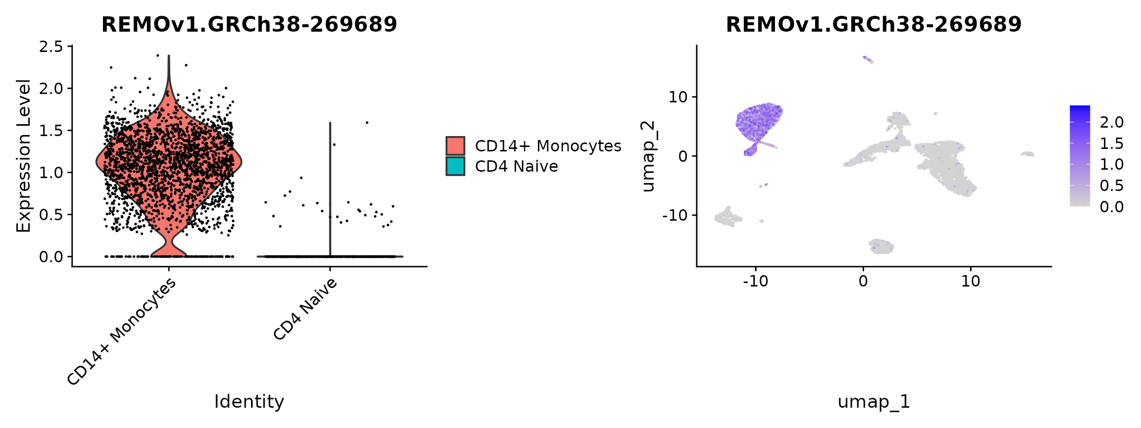
Cell type term enrichment
We can also perform an automated cell type annotation using the REMO cell type ontology terms, through an ontology term enrichment analysis. This is useful if we don’t have access to an annotated reference dataset for label transfer, or to provide additional cell type predictions independent of reference mapping.
Here we demonstrate how to perform CL term enrichment analysis for each cell cluster using REMO and the fgsea package.
if (!requireNamespace("fgsea", quietly = TRUE)) {
  BiocManager::install("fgsea")
}
We can use the EnrichedTerms() function in Signac to run
ontology enrichment on a ranked list of features for each cluster. We
need to provide a list of ontology terms associated with each feature in
our assay. For REMO, this is included in the
REMO.v1.GRCh38.terms object included in the package. We can
subset these terms to only include cell types in a tissue that we’re
interested in using the included list of tissue-celltype
associations:
celltypes <- REMO.v1.GRCh38.terms[REMO.v1.GRCh38.tissues$Blood]
enrichments <- EnrichedTerms(
  object = pbmc,
  terms = celltypes,
  group.by = "seurat_clusters",
  verbose = FALSE
)
For each cluster we have a list of potential cell type names and the strength of their enrichment. We can explore these for each cluster in detail, but as an initial check let’s assign each cluster to the top celltype term:
new_ids <- sapply(enrichments, function(df) df$pathway[1])
new_ids[is.na(new_ids)] <- "unknown"
Idents(pbmc) <- "seurat_clusters"
pbmc <- RenameIdents(pbmc, new_ids)
plot5 <- DimPlot(pbmc, label = TRUE, repel = TRUE) + NoLegend() + ggtitle("CL enrichment")

plot2 + ggtitle("Label transfer") | plot5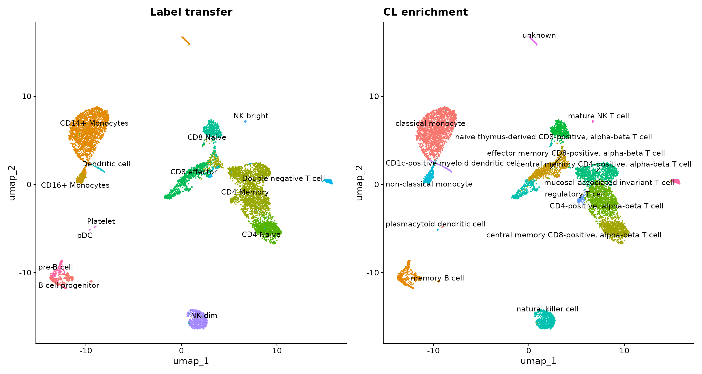
As we can see, many of the cell type predictions for our REMO clusters match the label transfer results. However, some do not. It’s important to inspect these results and combine with other sources of information (gene activity of cell type marker genes, for example) to decide on a final cell type label assignment.
Plotting genomic regions
We can plot the frequency of Tn5 integration across regions of the
genome for cells grouped by cluster, cell type, or any other metadata
stored in the object for any genomic region using the
CoveragePlot() function. These represent pseudo-bulk
accessibility tracks, where signal from all cells within a group have
been averaged together to visualize the DNA accessibility in a region.
Alongside these accessibility tracks we can visualize other important
information including gene annotation, peak coordinates, and genomic
links (if they’re stored in the object). See the visualization vignette for more
information.
For plotting purposes, it’s nice to have related cell types grouped
together. We can automatically sort the plotting order according to
similarities across the annotated cell types by running the
SortIdents() function:
Idents(pbmc) <- "predicted.id"
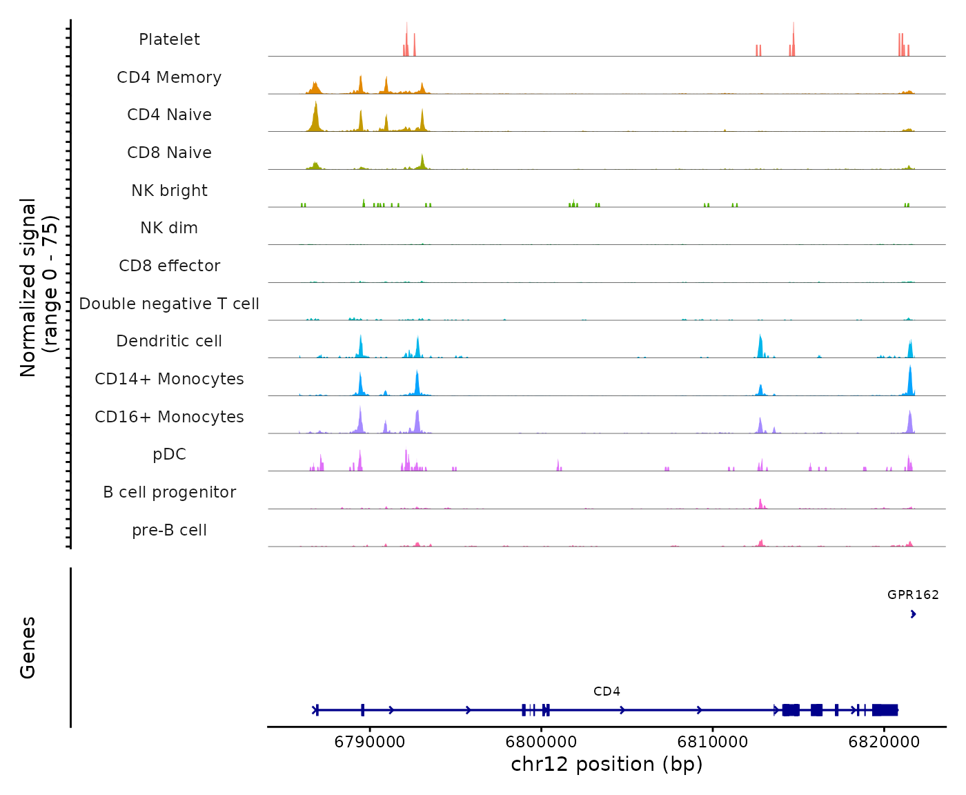
pbmc <- SortIdents(pbmc)We can then visualize the DNA accessibility in different genomic
regions using the CoveragePlot() function:
CoveragePlot(
  object = pbmc,
  region = "CD4",
  extend.upstream = 1000,
  extend.downstream = 1000
)
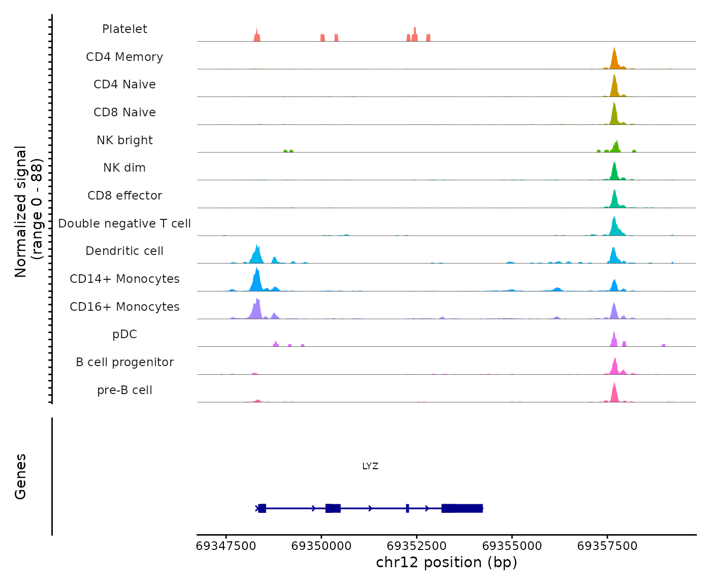
CoveragePlot(
  object = pbmc,
  region = "LYZ",
  extend.upstream = 1000,
  extend.downstream = 5000
)
Session Info
## R version 4.5.0 (2025-04-11)
## Platform: x86_64-pc-linux-gnu
## Running under: Red Hat Enterprise Linux 8.10 (Ootpa)
##
## Matrix products: default
## BLAS:   /charonfs/home/users/astar/gis/stuartt/R-4.5.0/lib/libRblas.so
## LAPACK: /charonfs/home/users/astar/gis/stuartt/R-4.5.0/lib/libRlapack.so;  LAPACK version 3.12.1
##
## locale:
##  [1] LC_CTYPE=en_US.UTF-8       LC_NUMERIC=C               LC_TIME=en_US.UTF-8        LC_COLLATE=en_US.UTF-8     LC_MONETARY=en_US.UTF-8    LC_MESSAGES=en_US.UTF-8    LC_PAPER=en_US.UTF-8       LC_NAME=C                  LC_ADDRESS=C               LC_TELEPHONE=C             LC_MEASUREMENT=en_US.UTF-8 LC_IDENTIFICATION=C
##
## time zone: Asia/Singapore
## tzcode source: system (glibc)
##
## attached base packages:
## [1] stats4    stats     graphics  grDevices utils     datasets  methods   base
##
## other attached packages:
##  [1] scDblFinder_1.24.10         SingleCellExperiment_1.32.0 SummarizedExperiment_1.40.0 MatrixGenerics_1.22.0       matrixStats_1.5.0           REMO.v1.GRCh38_1.0.0        enrichplot_1.30.5           org.Hs.eg.db_3.22.0         clusterProfiler_4.18.4      future_1.70.0               ensembldb_2.34.0            AnnotationFilter_1.34.0     GenomicFeatures_1.62.0      AnnotationDbi_1.72.0        Biobase_2.70.0              AnnotationHub_4.0.0         BiocFileCache_3.0.0         dbplyr_2.5.2                dplyr_1.2.0                 GenomeInfoDb_1.46.2         patchwork_1.3.2
## [22] ggplot2_4.0.2               GenomicRanges_1.62.1        Seqinfo_1.0.0               IRanges_2.44.0              S4Vectors_0.48.0            BiocGenerics_0.56.0         generics_0.1.4              Seurat_5.4.0                SeuratObject_5.3.0          sp_2.2-1                    Signac_1.9999.0
##
## loaded via a namespace (and not attached):
##   [1] R.methodsS3_1.8.2        dichromat_2.0-0.1        nnet_7.3-20              goftest_1.2-3            Biostrings_2.78.0        vctrs_0.7.1              ggtangle_0.1.1           spatstat.random_3.4-4    digest_0.6.39            png_0.1-9                ggrepel_0.9.7            deldir_2.0-4             parallelly_1.46.1        MASS_7.3-65              fontLiberation_0.1.0     pkgdown_2.2.0            reshape2_1.4.5           httpuv_1.6.16            qvalue_2.42.0            withr_3.0.2              ggrastr_1.0.2            xfun_0.56                ggfun_0.2.0
##  [24] survival_3.8-6           memoise_2.0.1            ggbeeswarm_0.7.3         gson_0.1.0               systemfonts_1.3.2        ragg_1.5.0               tidytree_0.4.7           zoo_1.8-15               pbapply_1.7-4            R.oo_1.27.1              Formula_1.2-5            KEGGREST_1.50.0          promises_1.5.0           otel_0.2.0               httr_1.4.8               restfulr_0.0.16          globals_0.19.1           fitdistrplus_1.2-6       stringfish_0.18.0        rstudioapi_0.18.0        UCSC.utils_1.6.1         miniUI_0.1.2             DOSE_4.4.0
##  [47] base64enc_0.1-6          curl_7.0.0               fields_17.1              ScaledMatrix_1.18.0      polyclip_1.10-7          SparseArray_1.10.8       xtable_1.8-8             stringr_1.6.0            desc_1.4.3               evaluate_1.0.5           S4Arrays_1.10.1          irlba_2.3.7              colorspace_2.1-2         filelock_1.0.3           hdf5r_1.3.12             ROCR_1.0-12              qs2_0.1.7                reticulate_1.45.0        spatstat.data_3.1-9      magrittr_2.0.4           lmtest_0.9-40            viridis_0.6.5            later_1.4.8
##  [70] ggtree_4.0.4             lattice_0.22-9           spatstat.geom_3.7-0      future.apply_1.20.2      scuttle_1.20.0           scattermore_1.2          XML_3.99-0.23            cowplot_1.2.0            RcppAnnoy_0.0.23         Hmisc_5.2-5              pillar_1.11.1            nlme_3.1-168             beachmat_2.26.0          compiler_4.5.0           RSpectra_0.16-2          stringi_1.8.7            tensor_1.5.1             GenomicAlignments_1.46.0 plyr_1.8.9               scater_1.38.0            crayon_1.5.3             abind_1.4-8              BiocIO_1.20.0
##  [93] gridGraphics_0.5-1       locfit_1.5-9.12          bit_4.6.0                fastmatch_1.1-8          codetools_0.2-20         textshaping_1.0.4        BiocSingular_1.26.1      bslib_0.10.0             biovizBase_1.58.0        plotly_4.12.0            mime_0.13                splines_4.5.0            Rcpp_1.1.1               fastDummies_1.7.5        tidydr_0.0.6             sparseMatrixStats_1.22.0 knitr_1.51               blob_1.3.0               BiocVersion_3.22.0       fs_1.6.7                 listenv_0.10.1           checkmate_2.3.4          ggplotify_0.1.3
## [116] tibble_3.3.1             Matrix_1.7-4             statmod_1.5.1            tweenr_2.0.3             pkgconfig_2.0.3          tools_4.5.0              cachem_1.1.0             cigarillo_1.0.0          RSQLite_2.4.6            viridisLite_0.4.3        DBI_1.3.0                fastmap_1.2.0            rmarkdown_2.30           scales_1.4.0             grid_4.5.0               ica_1.0-3                Rsamtools_2.26.0         sass_0.4.10              BiocManager_1.30.27      dotCall64_1.2            VariantAnnotation_1.56.0 RANN_2.6.2               rpart_4.1.24
## [139] farver_2.1.2             scatterpie_0.2.6         yaml_2.3.12              foreign_0.8-91           rtracklayer_1.70.1       cli_3.6.5                purrr_1.2.1              lifecycle_1.0.5          uwot_0.2.4               bluster_1.20.0           presto_1.0.0             backports_1.5.0          BiocParallel_1.44.0      gtable_0.3.6             rjson_0.2.23             ggridges_0.5.7           progressr_0.18.0         parallel_4.5.0           ape_5.8-1                limma_3.66.0             edgeR_4.8.2              jsonlite_2.0.0           RcppHNSW_0.6.0
## [162] bitops_1.0-9             xgboost_3.2.0.1          bit64_4.6.0-1            Rtsne_0.17               yulab.utils_0.2.4        BiocNeighbors_2.4.0      spatstat.utils_3.2-1     RcppParallel_5.1.11-1    metapod_1.18.0           jquerylib_0.1.4          dqrng_0.4.1              GOSemSim_2.36.0          spatstat.univar_3.1-6    R.utils_2.13.0           lazyeval_0.2.2           shiny_1.13.0             htmltools_0.5.9          GO.db_3.22.0             sctransform_0.4.3        rappdirs_0.3.4           glue_1.8.0               spam_2.11-3              httr2_1.2.2
## [185] XVector_0.50.0           gdtools_0.5.0            RCurl_1.98-1.17          InteractionSet_1.38.0    treeio_1.34.0            scran_1.38.1             BSgenome_1.78.0          gridExtra_2.3            igraph_2.2.2             R6_2.6.1                 tidyr_1.3.2              ggiraph_0.9.6            RcppRoll_0.3.1           labeling_0.4.3           cluster_2.1.8.2          aplot_0.2.9              DelayedArray_0.36.0      tidyselect_1.2.1         vipor_0.4.7              ProtGenerics_1.42.0      htmlTable_2.4.3          maps_3.4.3               ggforce_0.5.0
## [208] fontBitstreamVera_0.1.1  rsvd_1.0.5               KernSmooth_2.23-26       S7_0.2.1                 fontquiver_0.2.1         data.table_1.18.2.1      htmlwidgets_1.6.4        fgsea_1.36.2             RColorBrewer_1.1-3       rlang_1.1.7              spatstat.sparse_3.1-0    spatstat.explore_3.7-0   ggnewscale_0.5.2         beeswarm_0.4.0