Analyzing adult mouse brain scATAC-seq
Compiled: March 20, 2026
Source:vignettes/mouse_brain_vignette.Rmd
mouse_brain_vignette.RmdFor this tutorial, we will be analyzing a single-cell ATAC-seq dataset of adult mouse brain cells provided by 10x Genomics. The following files are used in this vignette, all available through the 10x Genomics website.
View data download code
To download the required data, run the following lines in a shell:
wget http://cf.10xgenomics.com/samples/cell-atac/1.1.0/atac_v1_adult_brain_fresh_5k/atac_v1_adult_brain_fresh_5k_filtered_peak_bc_matrix.h5
wget http://cf.10xgenomics.com/samples/cell-atac/1.1.0/atac_v1_adult_brain_fresh_5k/atac_v1_adult_brain_fresh_5k_singlecell.csv
wget http://cf.10xgenomics.com/samples/cell-atac/1.1.0/atac_v1_adult_brain_fresh_5k/atac_v1_adult_brain_fresh_5k_fragments.tsv.gz
wget http://cf.10xgenomics.com/samples/cell-atac/1.1.0/atac_v1_adult_brain_fresh_5k/atac_v1_adult_brain_fresh_5k_fragments.tsv.gz.tbi
This vignette echoes the commands run in the introductory Signac vignette on human PBMC. We provide the same analysis in a different system to demonstrate performance and applicability to other tissue types, and to provide an example from another species.
First load in Signac, Seurat, and some other packages we will be using for analyzing mouse data.
Pre-processing workflow
counts <- Read10X_h5("atac_v1_adult_brain_fresh_5k_filtered_peak_bc_matrix.h5")
metadata <- read.csv(
  file = "atac_v1_adult_brain_fresh_5k_singlecell.csv",
  header = TRUE,
  row.names = 1
)

brain_assay <- CreateGRangesAssay(
  counts = counts,
  fragments = "atac_v1_adult_brain_fresh_5k_fragments.tsv.gz",
  min.cells = 1
)
## Computing hash
brain <- CreateSeuratObject(
  counts = brain_assay,
  assay = "peaks",
  project = "ATAC",
  meta.data = metadata
)
We can also add gene annotations to the brain object for
the mouse genome. This will allow downstream functions to pull the gene
annotation information directly from the object.
# extract gene annotations from EnsDb
annotations <- GetGRangesFromEnsDb(ensdb = EnsDb.Mmusculus.v79)

# change to UCSC style since the data was mapped to mm10
seqlevels(annotations) <- paste0("chr", seqlevels(annotations))
genome(annotations) <- "mm10"

# add the gene information to the object
Annotation(brain) <- annotations
Computing QC Metrics
Next we compute some useful per-cell QC metrics including the
nucleosome signal, TSS enrichment score, and total counts per cell using
the ATACqc() function:
brain <- ATACqc(brain)
VlnPlot(
  object = brain,
  features = c("total_fragments", "TSS_enrichment", "Nucleosome_signal", "FRiP"),
  pt.size = 0.1,
  ncol = 5
)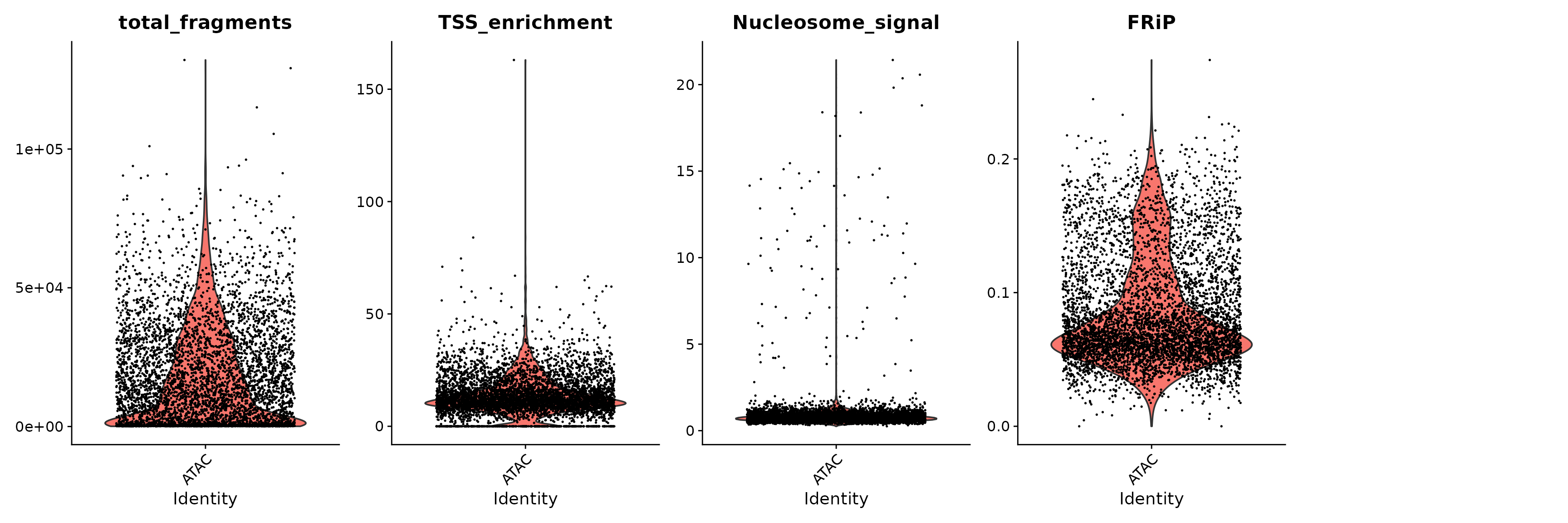
We remove cells that are outliers for these QC metrics.
brain <- subset(
  x = brain,
  subset = total_fragments > 3000 &
    total_fragments < 100000 &
    Nucleosome_signal < 4 &
    TSS_enrichment > 7
)
brain
## An object of class Seurat
## 157203 features across 3562 samples within 1 assay
## Active assay: peaks (157203 features, 0 variable features)
## 1 layer present: countsNormalization and linear dimensional reduction
brain <- RunTFIDF(brain)
brain <- FindTopFeatures(brain, min.cutoff = "q0")
brain <- RunSVD(object = brain)
The first LSI component often captures sequencing depth (technical
variation) rather than biological variation. If this is the case, the
component should be removed from downstream analysis. We can assess the
correlation between each LSI component and sequencing depth using the
DepthCor() function:
DepthCor(brain)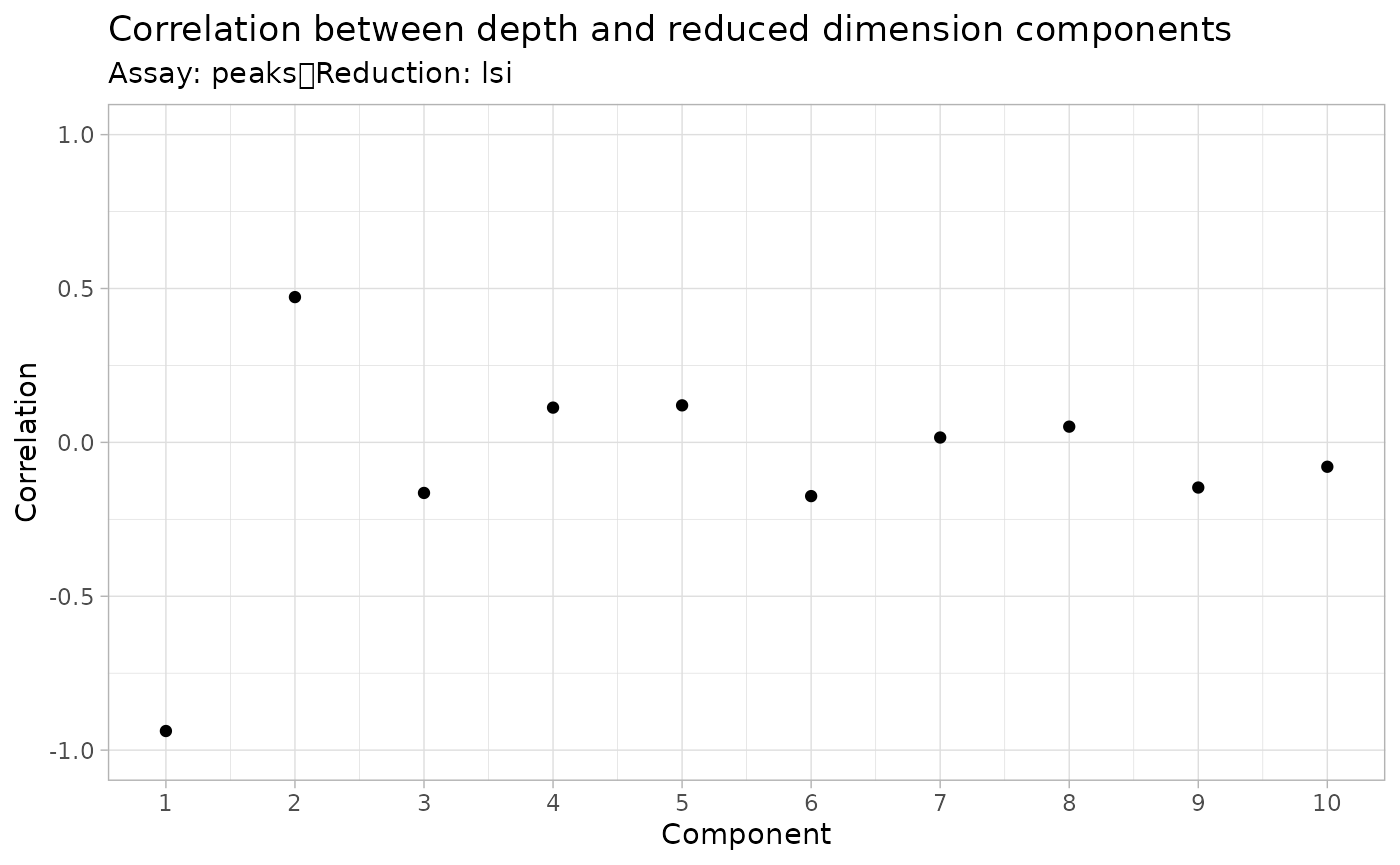
Here we see there is a very strong correlation between the first LSI component and the total number of counts for the cell, so we will perform downstream steps without this component.
Non-linear dimension reduction and clustering
Now that the cells are embedded in a low-dimensional space, we can
use methods commonly applied for the analysis of scRNA-seq data to
perform graph-based clustering, and non-linear dimension reduction for
visualization. The functions RunUMAP(),
FindNeighbors(), and FindClusters() all come
from the Seurat package.
brain <- RunUMAP(
  object = brain,
  reduction = "lsi",
  dims = 2:30
)
brain <- FindNeighbors(
  object = brain,
  reduction = "lsi",
  dims = 2:30
)
brain <- FindClusters(
  object = brain,
  algorithm = 3,
  resolution = 1.2,
  verbose = FALSE
)

DimPlot(object = brain, label = TRUE) + NoLegend()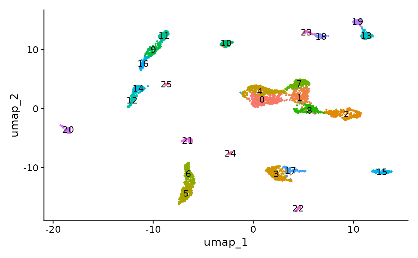
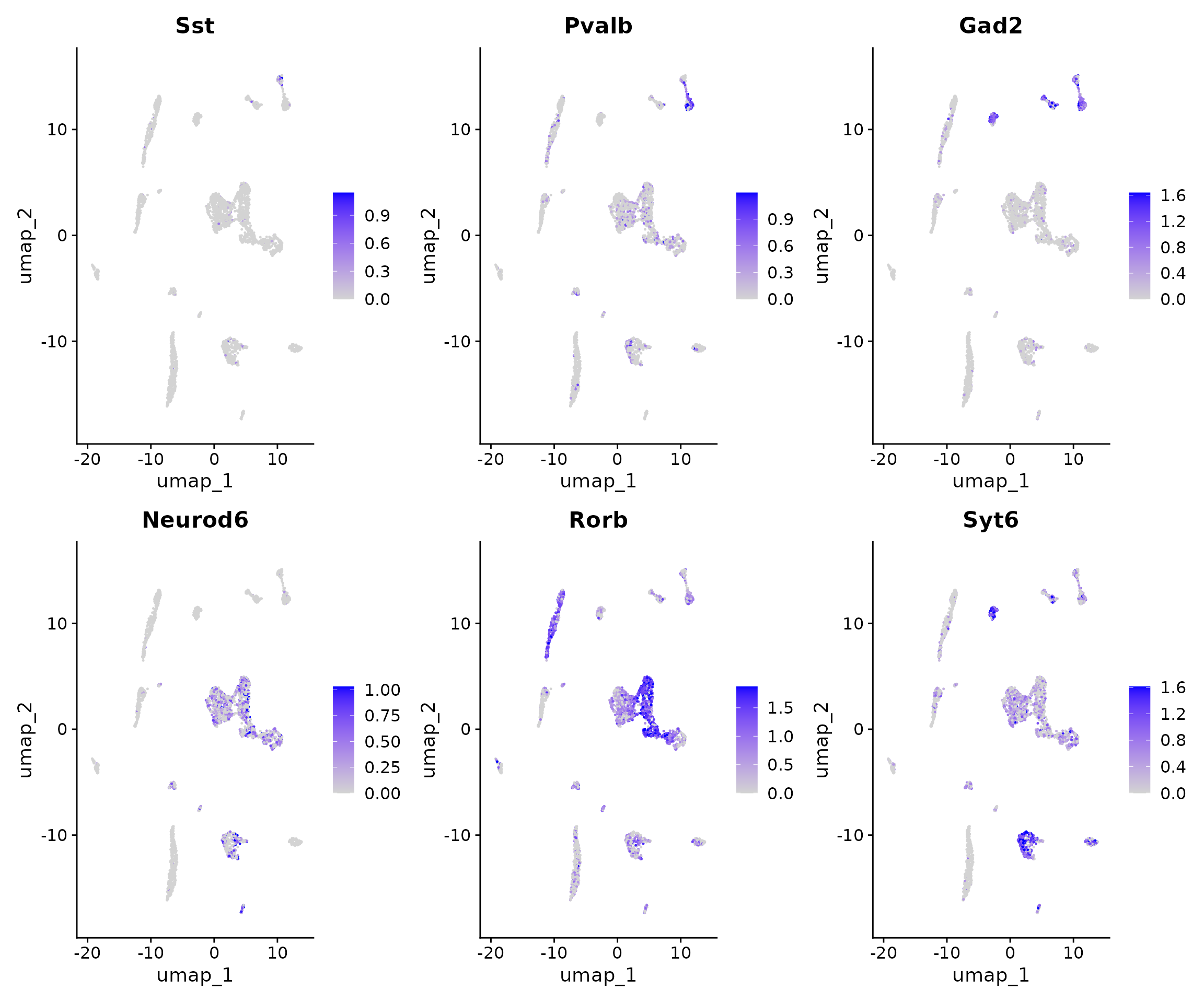
Create a gene activity matrix
# compute gene activities
gene.activities <- GeneActivity(brain)

# add the gene activity matrix to the Seurat object as a new assay
brain[["RNA"]] <- CreateAssay5Object(counts = gene.activities)
brain <- NormalizeData(brain, assay = "RNA")
DefaultAssay(brain) <- "RNA"
FeaturePlot(
  object = brain,
  features = c("Sst", "Pvalb", "Gad2", "Neurod6", "Rorb", "Syt6"),
  pt.size = 0.1,
  max.cutoff = "q95",
  ncol = 3
)
Integrating with scRNA-seq data
To help interpret the scATAC-seq data, we can classify cells based on an scRNA-seq experiment from the same biological system (the adult mouse brain). We utilize methods for cross-modality integration and label transfer, described here, with a more in-depth tutorial here.
You can download the raw data for this experiment from the Allen Institute website, and view the code used to construct this object on GitHub. Alternatively, you can download the pre-processed Seurat object here.
# Load the pre-processed scRNA-seq data
allen_rna <- readRDS("allen_brain.rds")
allen_rna <- UpdateSeuratObject(allen_rna)
allen_rna <- FindVariableFeatures(
  object = allen_rna,
  nfeatures = 5000
)

transfer.anchors <- FindTransferAnchors(
  reference = allen_rna,
  query = brain,
  reduction = "cca",
  dims = 1:30
)

predicted.labels <- TransferData(
  anchorset = transfer.anchors,
  refdata = allen_rna$subclass,
  weight.reduction = brain[["lsi"]],
  dims = 2:30
)

brain <- AddMetaData(object = brain, metadata = predicted.labels)
plot1 <- DimPlot(allen_rna, group.by = "subclass", label = TRUE, repel = TRUE) + NoLegend() + ggtitle("scRNA-seq")
plot2 <- DimPlot(brain, group.by = "predicted.id", label = TRUE, repel = TRUE) + NoLegend() + ggtitle("scATAC-seq")
plot1 + plot2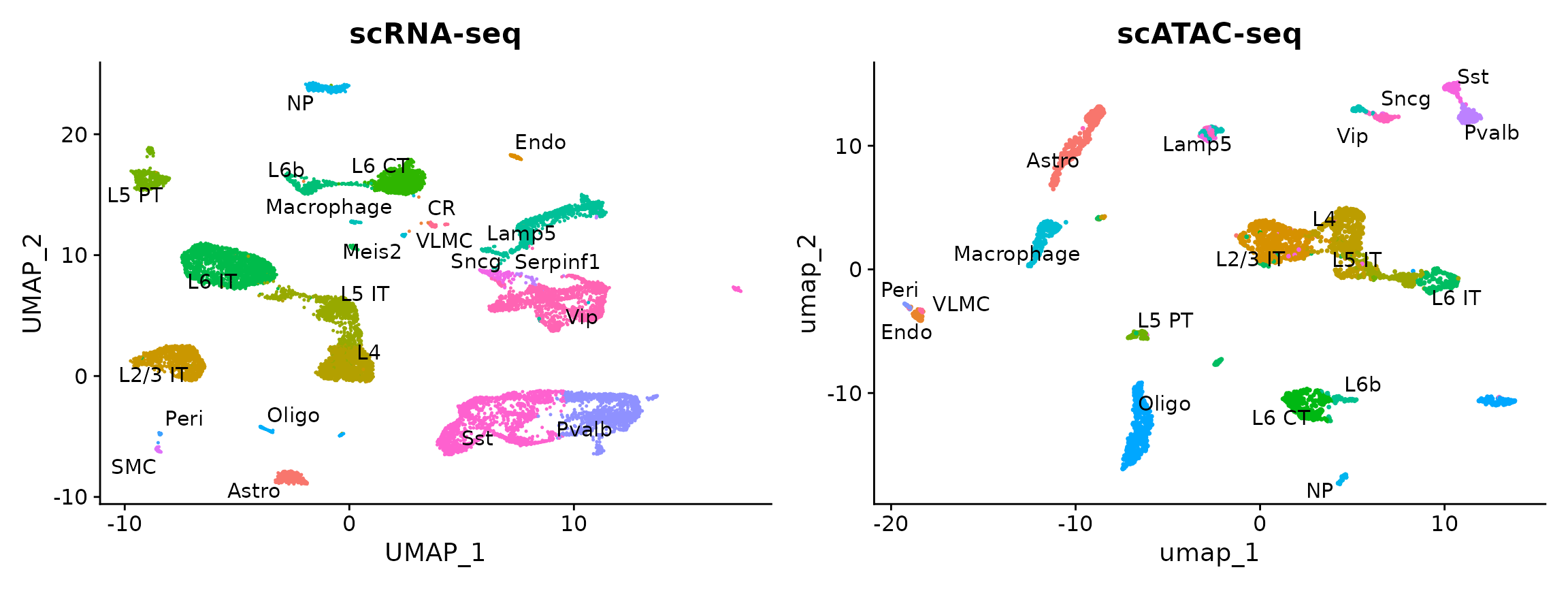
You can see that the RNA-based classifications are consistent with the UMAP visualization, computed only on the ATAC-seq data.
Find differentially accessible peaks between clusters
Here, we find differentially accessible regions between excitatory neurons in different layers of the cortex.
# switch back to working with peaks instead of gene activities
DefaultAssay(brain) <- "peaks"
Idents(brain) <- "predicted.id"

da_peaks <- FindMarkers(
  object = brain,
  ident.1 = c("L2/3 IT"),
  ident.2 = c("L4", "L5 IT", "L6 IT"),
  test.use = "wilcox",
  min.pct = 0.1
)

head(da_peaks)
## p_val avg_log2FC pct.1 pct.2 p_val_adj
## chr4:86523678-86525285 6.084182e-82 3.915105 0.419 0.032 9.564517e-77
## chr2:118700082-118704897 4.103277e-78 2.096779 0.637 0.174 6.450475e-73
## chr15:87605281-87607659 4.077245e-69 2.500735 0.491 0.092 6.409551e-64
## chr3:137056475-137058371 1.420958e-68 2.260298 0.525 0.110 2.233788e-63
## chr10:107751762-107753240 2.401929e-68 1.889627 0.623 0.179 3.775905e-63
## chr4:101303935-101305131 1.621729e-67 3.857710 0.349 0.023 2.549407e-62
plot1 <- VlnPlot(
  object = brain,
  features = rownames(da_peaks)[1],
  pt.size = 0.1,
  idents = c("L4", "L5 IT", "L2/3 IT")
)
plot2 <- FeaturePlot(
  object = brain,
  features = rownames(da_peaks)[1],
  pt.size = 0.1,
  max.cutoff = "q95"
)
plot1 | plot2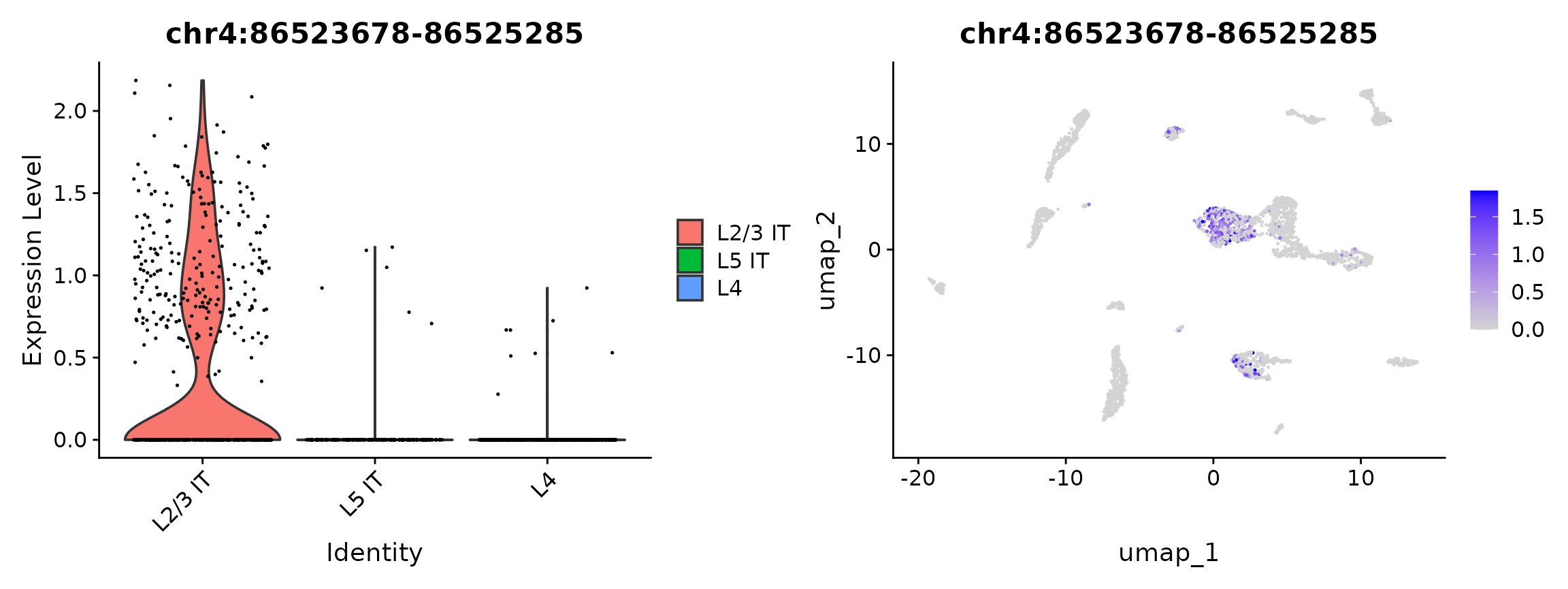
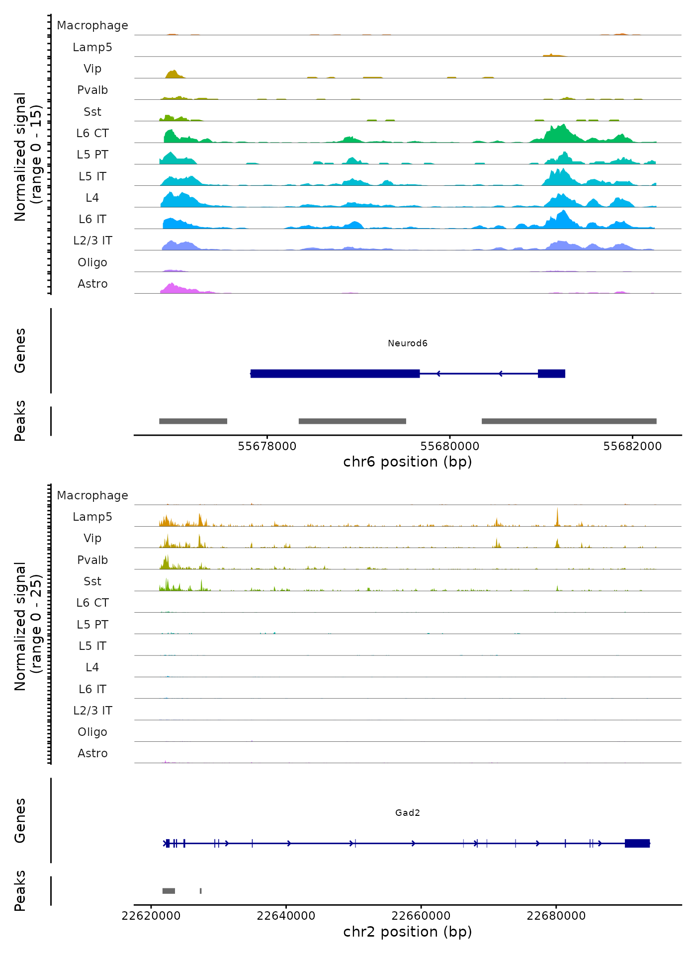
Plotting genomic regions
We can also create coverage plots grouped by cluster, cell type, or
any other metadata stored in the object for any genomic region using the
CoveragePlot() function. These represent pseudo-bulk
accessibility tracks, where signal from all cells within a group have
been averaged together to visualize the DNA accessibility in a
region.
# show cell types with at least 50 cells
idents.plot <- names(which(table(Idents(brain)) > 50))
brain <- SortIdents(brain)

CoveragePlot(
  object = brain,
  region = c("Neurod6", "Gad2"),
  idents = idents.plot,
  extend.upstream = 1000,
  extend.downstream = 1000,
  ncol = 1
)
Session Info
## R version 4.5.0 (2025-04-11)
## Platform: x86_64-pc-linux-gnu
## Running under: Red Hat Enterprise Linux 8.10 (Ootpa)
##
## Matrix products: default
## BLAS:   /charonfs/home/users/astar/gis/stuartt/R-4.5.0/lib/libRblas.so
## LAPACK: /charonfs/home/users/astar/gis/stuartt/R-4.5.0/lib/libRlapack.so;  LAPACK version 3.12.1
##
## locale:
##  [1] LC_CTYPE=en_US.UTF-8       LC_NUMERIC=C
##  [3] LC_TIME=en_US.UTF-8        LC_COLLATE=en_US.UTF-8
##  [5] LC_MONETARY=en_US.UTF-8    LC_MESSAGES=en_US.UTF-8
##  [7] LC_PAPER=en_US.UTF-8       LC_NAME=C
##  [9] LC_ADDRESS=C               LC_TELEPHONE=C
## [11] LC_MEASUREMENT=en_US.UTF-8 LC_IDENTIFICATION=C
##
## time zone: Asia/Singapore
## tzcode source: system (glibc)
##
## attached base packages:
## [1] stats4    stats     graphics  grDevices utils     datasets  methods
## [8] base
##
## other attached packages:
##  [1] future_1.70.0              patchwork_1.3.2
##  [3] ggplot2_4.0.2              EnsDb.Mmusculus.v79_2.99.0
##  [5] ensembldb_2.34.0           AnnotationFilter_1.34.0
##  [7] GenomicFeatures_1.62.0     AnnotationDbi_1.72.0
##  [9] Biobase_2.70.0             GenomicRanges_1.62.1
## [11] Seqinfo_1.0.0              IRanges_2.44.0
## [13] S4Vectors_0.48.0           BiocGenerics_0.56.0
## [15] generics_0.1.4             Seurat_5.4.0
## [17] SeuratObject_5.3.0         sp_2.2-1
## [19] Signac_1.9999.0
##
## loaded via a namespace (and not attached):
##   [1] fs_1.6.7                    ProtGenerics_1.42.0
##   [3] matrixStats_1.5.0           spatstat.sparse_3.1-0
##   [5] bitops_1.0-9                httr_1.4.8
##   [7] RColorBrewer_1.1-3          InteractionSet_1.38.0
##   [9] tools_4.5.0                 sctransform_0.4.3
##  [11] backports_1.5.0             R6_2.6.1
##  [13] lazyeval_0.2.2              uwot_0.2.4
##  [15] withr_3.0.2                 gridExtra_2.3
##  [17] progressr_0.18.0            cli_3.6.5
##  [19] textshaping_1.0.4           spatstat.explore_3.7-0
##  [21] fastDummies_1.7.5           labeling_0.4.3
##  [23] sass_0.4.10                 S7_0.2.1
##  [25] spatstat.data_3.1-9         ggridges_0.5.7
##  [27] pbapply_1.7-4               pkgdown_2.2.0
##  [29] Rsamtools_2.26.0            systemfonts_1.3.2
##  [31] foreign_0.8-91              dichromat_2.0-0.1
##  [33] parallelly_1.46.1           BSgenome_1.78.0
##  [35] limma_3.66.0                rstudioapi_0.18.0
##  [37] RSQLite_2.4.6               BiocIO_1.20.0
##  [39] ica_1.0-3                   spatstat.random_3.4-4
##  [41] dplyr_1.2.0                 Matrix_1.7-4
##  [43] ggbeeswarm_0.7.3            abind_1.4-8
##  [45] lifecycle_1.0.5             yaml_2.3.12
##  [47] SummarizedExperiment_1.40.0 SparseArray_1.10.8
##  [49] Rtsne_0.17                  grid_4.5.0
##  [51] blob_1.3.0                  promises_1.5.0
##  [53] crayon_1.5.3                miniUI_0.1.2
##  [55] lattice_0.22-9              cowplot_1.2.0
##  [57] cigarillo_1.0.0             KEGGREST_1.50.0
##  [59] pillar_1.11.1               knitr_1.51
##  [61] rjson_0.2.23                future.apply_1.20.2
##  [63] codetools_0.2-20            fastmatch_1.1-8
##  [65] glue_1.8.0                  spatstat.univar_3.1-6
##  [67] data.table_1.18.2.1         vctrs_0.7.1
##  [69] png_0.1-9                   spam_2.11-3
##  [71] gtable_0.3.6                cachem_1.1.0
##  [73] xfun_0.56                   S4Arrays_1.10.1
##  [75] mime_0.13                   survival_3.8-6
##  [77] RcppRoll_0.3.1              statmod_1.5.1
##  [79] fitdistrplus_1.2-6          ROCR_1.0-12
##  [81] nlme_3.1-168                bit64_4.6.0-1
##  [83] RcppAnnoy_0.0.23            GenomeInfoDb_1.46.2
##  [85] bslib_0.10.0                irlba_2.3.7
##  [87] vipor_0.4.7                 KernSmooth_2.23-26
##  [89] otel_0.2.0                  rpart_4.1.24
##  [91] colorspace_2.1-2            DBI_1.3.0
##  [93] Hmisc_5.2-5                 nnet_7.3-20
##  [95] ggrastr_1.0.2               tidyselect_1.2.1
##  [97] bit_4.6.0                   compiler_4.5.0
##  [99] curl_7.0.0                  htmlTable_2.4.3
## [101] hdf5r_1.3.12                desc_1.4.3
## [103] DelayedArray_0.36.0         plotly_4.12.0
## [105] stringfish_0.18.0           rtracklayer_1.70.1
## [107] checkmate_2.3.4             scales_1.4.0
## [109] lmtest_0.9-40               stringr_1.6.0
## [111] digest_0.6.39               goftest_1.2-3
## [113] spatstat.utils_3.2-1        presto_1.0.0
## [115] rmarkdown_2.30              XVector_0.50.0
## [117] htmltools_0.5.9             pkgconfig_2.0.3
## [119] base64enc_0.1-6             sparseMatrixStats_1.22.0
## [121] MatrixGenerics_1.22.0       fastmap_1.2.0
## [123] rlang_1.1.7                 htmlwidgets_1.6.4
## [125] UCSC.utils_1.6.1            shiny_1.13.0
## [127] farver_2.1.2                jquerylib_0.1.4
## [129] zoo_1.8-15                  jsonlite_2.0.0
## [131] BiocParallel_1.44.0         VariantAnnotation_1.56.0
## [133] RCurl_1.98-1.17             magrittr_2.0.4
## [135] Formula_1.2-5               dotCall64_1.2
## [137] Rcpp_1.1.1                  reticulate_1.45.0
## [139] stringi_1.8.7               MASS_7.3-65
## [141] plyr_1.8.9                  parallel_4.5.0
## [143] listenv_0.10.1              ggrepel_0.9.7
## [145] deldir_2.0-4                Biostrings_2.78.0
## [147] splines_4.5.0               tensor_1.5.1
## [149] igraph_2.2.2                spatstat.geom_3.7-0
## [151] RcppHNSW_0.6.0              qs2_0.1.7
## [153] reshape2_1.4.5              XML_3.99-0.23
## [155] evaluate_1.0.5              biovizBase_1.58.0
## [157] RcppParallel_5.1.11-1       httpuv_1.6.16
## [159] RANN_2.6.2                  tidyr_1.3.2
## [161] purrr_1.2.1                 polyclip_1.10-7
## [163] scattermore_1.2             xtable_1.8-8
## [165] restfulr_0.0.16             RSpectra_0.16-2
## [167] later_1.4.8                 viridisLite_0.4.3
## [169] ragg_1.5.0                  tibble_3.3.1
## [171] memoise_2.0.1               beeswarm_0.4.0
## [173] GenomicAlignments_1.46.0    cluster_2.1.8.2
## [175] globals_0.19.1