
Large-scale scATAC-seq analysis with REMO and BPCells
Compiled: July 30, 2026
Source:vignettes/fetal_remo.Rmd
fetal_remo.RmdView data download code
In this tutorial we will demonstrate how large-scale scATAC-seq datasets from a variety of organs can be efficiently analyzed using Signac with a small memory footprint. This vignette analzying >620,000 cells was run on a Macbook Pro laptop with 16 Gb RAM.
First load in Signac, Seurat, and some other packages we will be using for analyzing human data.
## Warning: package 'Seurat' was built under R version 4.5.2## Warning: package 'SeuratObject' was built under R version 4.5.2## Warning: package 'sp' was built under R version 4.5.2## Warning: package 'GenomicRanges' was built under R version 4.5.2## Warning: package 'S4Vectors' was built under R version 4.5.3## Warning: package 'ggplot2' was built under R version 4.5.2Pre-processing workflow
When pre-processing chromatin data, Signac uses the ATAC fragment file as the main input data. This represents a full list of all unique fragments across all single cells. It is stored on-disk for memory efficiency and scalability. More information about the fragment file can be found on the 10x Genomics website or on the sinto website.
For improved scalability we will use our recently-released REMO features for the human genome, and store these features on-disk using BPCells.
You can install REMO and BPCells from GitHub:
remotes::install_github(repo = "stuart-lab/REMO.v1.GRCh38")
remotes::install_github("bnprks/BPCells/r")We start by identifying a set of cell barcodes to include in the
analysis by running the ATACqc() function on the fragment
file:
# load gene annotations for hg38
library(AnnotationHub)
ah <- AnnotationHub()

ensdb_v98 <- ah[["AH75011"]]
annotations <- GetGRangesFromEnsDb(ensdb = ensdb_v98)
seqlevelsStyle(annotations) <- "UCSC"

qc <- ATACqc(object = "fragments.tsv.gz", annotations = annotations)
# calculate knee plot using DropletUtils
br <- DropletUtils::barcodeRanks(matrix(qc$total_fragments, nrow = 1))
df <- as.data.frame(br)
knee <- S4Vectors::metadata(br)$knee

ggplot(df, aes(rank, total)) +
  geom_line() +
  geom_hline(yintercept = knee, linetype = "dashed") +
  annotate("text", x = 1, y = knee, label = paste0("knee = ", round(knee)),
           hjust = 0, vjust = -0.5) +
  scale_x_log10() + scale_y_log10() +
  xlab("Barcode rank") + ylab("Total fragments") +
  theme_bw()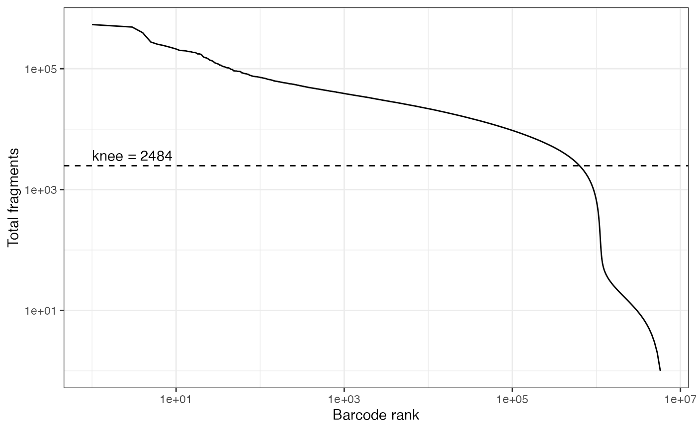
Next we can quantify REMO features for the selected cells using the
FeatureMatrix() function in Signac, storing the resulting
matrix on-disk using BPCells by setting bpcells=TRUE:
cells.use <- rownames(qc)[qc$total_fragments > knee]

counts <- FeatureMatrix(
  object = "fragments.tsv.gz",
  cells = cells.use,
  features = REMO.v1.GRCh38,
  group = TRUE,
  bpcells = TRUE,
  bpcells.dir = "./bpcells_counts"
)
## Grouping regions by column: REMO## Loading count matrixCreating the Seurat object
Next we initialize a Seurat object to store the data, using the
Signac ChromatinAssay5 assay class:
chrom_assay <- CreateChromatinAssay5(
  counts = counts,
  fragments = "fragments.tsv.gz",
  annotation = annotations,
  min.cells = 20
)
## Computing hash
fetal <- CreateSeuratObject(
  counts = chrom_assay,
  assay = "REMO",
  names.field = 2,
  names.delim = "__",
  meta.data = qc
)
fetal## An object of class Seurat
## 338933 features across 629666 samples within 1 assay
## Active assay: REMO (338933 features, 0 variable features)
## 1 layer present: countsDespite containing a large number of cells, we can see that the object requires less that 1 Gb of RAM due to storing the count matrix on disk:
format(object.size(fetal), "Gb")## [1] "0.9 Gb"Normalization and linear dimensional reduction
We proceed with standard feature selection, normalization, and PCA steps using the chromatin assay containing REMO features:
fetal <- FitMeanVar(fetal)## Finding variable features for layer counts## 338933 of 338933 features are eligible for selection after count filtering
fetal <- NormalizeData(fetal)## Normalizing layer: counts
fetal <- RunSVD(fetal, pca = TRUE)## Running PCANon-linear dimension reduction
Now that the cells are embedded in a low-dimensional space we project the cells into a two dimensional space for visualization using UMAP, and color the cells by their original tissue annotation.
fetal <- RunUMAP(object = fetal, dims = 1:50)

# extract original tissue annotations
fetal$tissue <- unlist(lapply(strsplit(as.character(fetal$orig.ident), "_SM-"), `[[`, 1))
DimPlot(fetal, group.by = "tissue", label = TRUE, raster = FALSE, repel = TRUE, pt.size = 0.1) + NoLegend()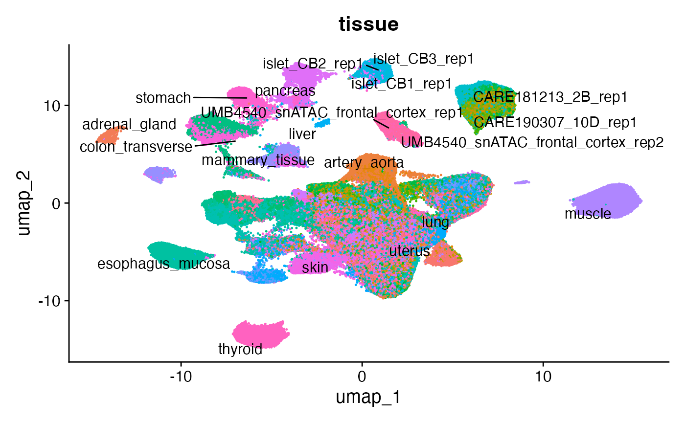
Plotting genomic regions
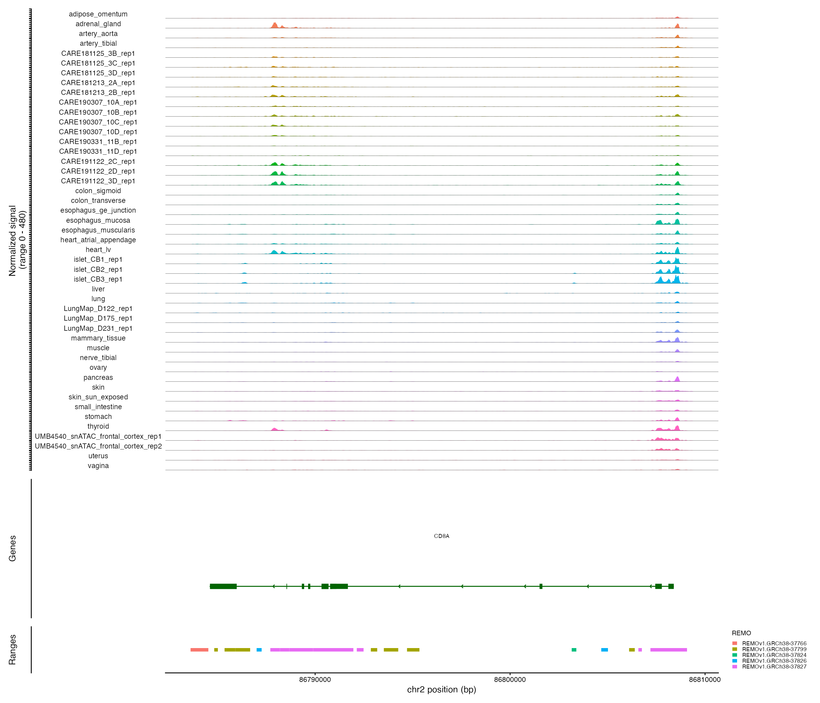
We can create genomic coverage plots for any region of the genome:
CoveragePlot(
  object = fetal,
  group.by = "tissue",
  region = "CD8A",
  ranges = REMO.v1.GRCh38,
  ranges.group.by = "REMO",
  extend.upstream = 1000,
  extend.downstream = 1000
)
Session Info
## R version 4.5.1 (2025-06-13)
## Platform: aarch64-apple-darwin20
## Running under: macOS Tahoe 26.5.2
##
## Matrix products: default
## BLAS:   /Library/Frameworks/R.framework/Versions/4.5-arm64/Resources/lib/libRblas.0.dylib
## LAPACK: /Library/Frameworks/R.framework/Versions/4.5-arm64/Resources/lib/libRlapack.dylib;  LAPACK version 3.12.1
##
## locale:
## [1] en_US.UTF-8/en_US.UTF-8/en_US.UTF-8/C/en_US.UTF-8/en_US.UTF-8
##
## time zone: Australia/Perth
## tzcode source: internal
##
## attached base packages:
## [1] stats4    stats     graphics  grDevices utils     datasets  methods   base
##
## other attached packages:
##  [1] ensembldb_2.34.0        AnnotationFilter_1.34.0 GenomicFeatures_1.62.0  AnnotationDbi_1.72.0    Biobase_2.70.0          AnnotationHub_4.0.0     BiocFileCache_3.0.0     dbplyr_2.6.0            BPCells_0.3.1           REMO.v1.GRCh38_1.0.0    ggplot2_4.0.3           GenomicRanges_1.62.1    Seqinfo_1.0.0           IRanges_2.44.0          S4Vectors_0.48.1        BiocGenerics_0.56.0     generics_0.1.4          Seurat_5.5.1            SeuratObject_5.4.0      sp_2.2-3                Signac_1.9999.6
##
## loaded via a namespace (and not attached):
##   [1] ProtGenerics_1.42.0         fs_2.1.0                    matrixStats_1.5.0           spatstat.sparse_3.2-0       bitops_1.0-9                httr_1.4.8                  RColorBrewer_1.1-3          InteractionSet_1.38.0       backports_1.5.1             tools_4.5.1                 sctransform_0.4.3           R6_2.6.1                    HDF5Array_1.38.0            lazyeval_0.2.3              uwot_0.2.4                  rhdf5filters_1.22.0         withr_3.0.3                 gridExtra_2.3.1             progressr_1.0.0             cli_3.6.6                   textshaping_1.0.5
##  [22] spatstat.explore_3.8-2      fastDummies_1.7.6           labeling_0.4.3              sass_0.4.10                 S7_0.2.2                    spatstat.data_3.1-9         ggridges_0.5.7              pbapply_1.7-4               pkgdown_2.2.1               Rsamtools_2.26.0            systemfonts_1.3.2           foreign_0.8-91              R.utils_2.13.0              dichromat_2.0-1             parallelly_1.48.0           BSgenome_1.78.0             limma_3.66.0                rstudioapi_0.19.0           RSQLite_3.53.3              BiocIO_1.20.0               ica_1.0-3
##  [43] spatstat.random_3.5-1       dplyr_1.2.1                 Matrix_1.7-6                abind_1.4-8                 R.methodsS3_1.8.2           lifecycle_1.0.5             yaml_2.3.12                 edgeR_4.8.2                 SummarizedExperiment_1.40.0 rhdf5_2.54.1                SparseArray_1.10.10         Rtsne_0.17                  grid_4.5.1                  blob_1.3.0                  promises_1.5.0              dqrng_0.4.1                 crayon_1.5.3                miniUI_0.1.2                lattice_0.22-9              beachmat_2.26.0             cowplot_1.2.0
##  [64] cigarillo_1.0.0             KEGGREST_1.50.0             pillar_1.11.1               knitr_1.51                  rjson_0.2.23                future.apply_1.20.2         codetools_0.2-20            fastmatch_1.1-8             glue_1.8.1                  spatstat.univar_3.2-0       data.table_1.18.4           vctrs_0.7.3                 png_0.1-9                   spam_2.11-4                 gtable_0.3.6                cachem_1.1.0                xfun_0.60                   S4Arrays_1.10.1             mime_0.13                   DropletUtils_1.30.0         survival_3.8-9
##  [85] SingleCellExperiment_1.32.0 RcppRoll_0.3.2              statmod_1.5.2               fitdistrplus_1.2-6          ROCR_1.0-12                 nlme_3.1-170                bit64_4.8.2                 filelock_1.0.3              RcppAnnoy_0.0.23            GenomeInfoDb_1.46.2         bslib_0.11.0                irlba_2.3.7                 rpart_4.1.27                KernSmooth_2.23-26          otel_0.2.0                  colorspace_2.1-3            Hmisc_5.2-6                 DBI_1.3.0                   nnet_7.3-20                 tidyselect_1.2.1            bit_4.6.0
## [106] compiler_4.5.1              curl_7.1.0                  httr2_1.3.0                 htmlTable_2.5.0             h5mread_1.2.1               desc_1.4.3                  DelayedArray_0.36.1         plotly_4.12.1               stringfish_0.19.0           rtracklayer_1.70.1          checkmate_2.3.4             scales_1.4.0                lmtest_0.9-40               rappdirs_0.3.4              stringr_1.6.0               digest_0.6.39               goftest_1.2-3               spatstat.utils_3.2-4        rmarkdown_2.31              XVector_0.50.0              base64enc_0.1-6
## [127] htmltools_0.5.9             pkgconfig_2.0.3             sparseMatrixStats_1.22.0    MatrixGenerics_1.22.0       fastmap_1.2.0               rlang_1.3.0                 htmlwidgets_1.6.4           UCSC.utils_1.6.1            shiny_1.14.0                DelayedMatrixStats_1.32.0   farver_2.1.2                jquerylib_0.1.4             zoo_1.8-15                  jsonlite_2.0.0              BiocParallel_1.44.0         R.oo_1.27.1                 VariantAnnotation_1.56.0    RCurl_1.98-1.19             magrittr_2.0.5              Formula_1.2-5               scuttle_1.20.0
## [148] dotCall64_1.2               patchwork_1.3.2             Rhdf5lib_1.32.0             Rcpp_1.1.2                  reticulate_1.46.0           stringi_1.8.7               MASS_7.3-66                 plyr_1.8.9                  parallel_4.5.1              listenv_1.0.0               ggrepel_0.9.8               deldir_2.0-4                Biostrings_2.78.0           splines_4.5.1               tensor_1.5.1                locfit_1.5-9.12             igraph_2.3.3                spatstat.geom_3.8-2         RcppHNSW_0.7.0              qs2_0.2.2                   reshape2_1.4.5
## [169] BiocVersion_3.22.0          XML_3.99-0.23               evaluate_1.0.5              biovizBase_1.58.0           RcppParallel_5.1.11-2       BiocManager_1.30.27         httpuv_1.6.17               RANN_2.6.2                  tidyr_1.3.2                 purrr_1.2.2                 polyclip_1.10-7             future_1.75.0               scattermore_1.2             xtable_1.8-8                restfulr_0.0.17             RSpectra_0.16-2             later_1.4.8                 viridisLite_0.4.3           ragg_1.5.2                  tibble_3.3.1                memoise_2.0.1
## [190] GenomicAlignments_1.46.0    cluster_2.1.8.2             globals_0.19.1