In this tutorial, we demonstrate how to call peaks on a single-cell ATAC-seq dataset using MACS3.
To use the peak calling functionality in Signac you will first need to install MACS3. This can be done using pip or conda, or by building the package from source.
MACS3 uses a dedicated parser for single-cell ATAC-seq fragment files, which contains the barcode information and the counts of the fragments aligned to the same location with the same barcode.
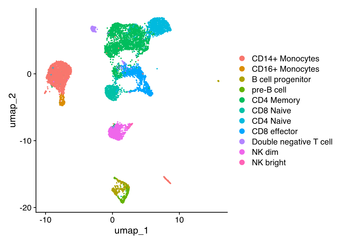
In this demonstration we use scATAC-seq data for human PBMCs. See our vignette for the code used to generate this object, and links to the raw data. First, load the required packages and the pre-computed Seurat object:
Peak calling with callpeak mode
Peak calling can be performed using the CallPeaks()
function on a Seurat object, ChromatinAssay5
object, Fragment2 object, or by giving the path to a
fragment file on disk.
## GRanges object with 6 ranges and 6 metadata columns:
##         seqnames        ranges strand |                 name     score
##            <Rle>     <IRanges>  <Rle> |          <character> <integer>
##   [1] GL000194.1   56039-56324      * | SeuratProject_peak_1      1290
##   [2] GL000194.1 101211-101818      * | SeuratProject_peak_2      3425
##   [3] GL000194.1 114384-115052      * | SeuratProject_peak_3      8293
##   [4] GL000195.1   24088-24460      * | SeuratProject_peak_4       269
##   [5] GL000195.1   24972-25447      * | SeuratProject_peak_5       101
##   [6] GL000195.1   30539-30907      * | SeuratProject_peak_6     43592
##       fold_change neg_log10pvalue_summit neg_log10qvalue_summit
##         <numeric>              <numeric>              <numeric>
##   [1]     8.36676               131.1970                129.027
##   [2]    15.41060               344.9850                342.510
##   [3]    28.31830               832.1450                829.313
##   [4]     3.71856                28.7884                 26.961
##   [5]     2.53863                11.8498                 10.180
##   [6]    21.13710              4363.3400               4359.280
##       relative_summit_position
##                      <integer>
##   [1]                       55
##   [2]                      142
##   [3]                      628
##   [4]                       67
##   [5]                      126
##   [6]                      303
##   -------
##   seqinfo: 35 sequences from an unspecified genome; no seqlengths
Parallelization across cell groups with future
We have observed that the runtime for MACS3 may be longer than
previous versions of MACS that reads in the input as a standard BED
file. When calling peaks across multiple groups of cells, we recommend
enabling parallelization in R using the future package (see
future::plan() for details on how to configure
parallelization). This will enable peaks to be called in parallel for
each group of cells.
library(future)

# set up workers
plan(multicore, workers = 6)
nbrOfWorkers()
## [1] 6To call peaks on each annotated cell type, we can use the
group.by argument:
peaks <- CallPeaks(pbmc, group.by = "predicted.id")The results are returned as a GRanges object, with an
additional metadata column listing the cell types that each peak was
identified in:
| seqnames | start | end | width | strand | peak_called_in |
|---|---|---|---|---|---|
| chr1 | 17334 | 17523 | 190 | * | NK bright |
| chr1 | 180771 | 180948 | 178 | * | CD4 Memory |
| chr1 | 191319 | 191882 | 564 | * | CD8 Naive,CD8 effector,CD14+ Monocytes,CD4 Naive |
| chr1 | 267818 | 268402 | 585 | * | CD4 Naive,pre-B cell |
| chr1 | 271259 | 271459 | 201 | * | CD14+ Monocytes |
| chr1 | 280585 | 280747 | 163 | * | CD16+ Monocytes |
To call peaks for specific group(s) of cells, use the
idents argument:
peaks <- CallPeaks(pbmc, group.by = "predicted.id", idents = "CD16+ Monocytes")By default, CallPeaks() will combine all peak calls into
one GRanges object. Set combine.peaks = FALSE
to return a list with a GRanges object for each group:
peaks_separate <- CallPeaks(
  object = pbmc,
  group.by = "predicted.id",
  idents = c("CD4 Naive", "CD4 Memory"),
  combine.peaks = FALSE
)| seqnames | start | end | width | strand | name | score | fold_change | neg_log10pvalue_summit | neg_log10qvalue_summit | relative_summit_position | ident |
|---|---|---|---|---|---|---|---|---|---|---|---|
| GL000194.1 | 56039 | 56285 | 247 | * | CD4_Memory1_peak_1 | 353 | 8.33203 | 37.55560 | 35.32860 | 36 | CD4 Memory |
| GL000194.1 | 101301 | 101540 | 240 | * | CD4_Memory1_peak_2 | 286 | 7.37590 | 30.81270 | 28.63380 | 169 | CD4 Memory |
| GL000194.1 | 114650 | 115052 | 403 | * | CD4_Memory1_peak_3 | 2605 | 31.41580 | 263.44000 | 260.56300 | 363 | CD4 Memory |
| GL000195.1 | 23147 | 23364 | 218 | * | CD4_Memory1_peak_4 | 32 | 2.73181 | 4.96328 | 3.20745 | 211 | CD4 Memory |
| GL000195.1 | 25038 | 25364 | 327 | * | CD4_Memory1_peak_5 | 90 | 4.09772 | 11.04690 | 9.09130 | 121 | CD4 Memory |
| GL000195.1 | 30545 | 30907 | 363 | * | CD4_Memory1_peak_6 | 12468 | 21.68910 | 1251.06000 | 1246.89000 | 298 | CD4 Memory |
| seqnames | start | end | width | strand | name | score | fold_change | neg_log10pvalue_summit | neg_log10qvalue_summit | relative_summit_position | ident |
|---|---|---|---|---|---|---|---|---|---|---|---|
| GL000194.1 | 114705 | 115039 | 335 | * | CD4_Naive1_peak_1 | 612 | 19.17440 | 63.97530 | 61.27650 | 308 | CD4 Naive |
| GL000195.1 | 24324 | 24631 | 308 | * | CD4_Naive1_peak_2 | 58 | 4.71501 | 7.91998 | 5.86784 | 29 | CD4 Naive |
| GL000195.1 | 25046 | 25202 | 157 | * | CD4_Naive1_peak_3 | 58 | 4.71501 | 7.91998 | 5.86784 | 78 | CD4 Naive |
| GL000195.1 | 30549 | 30908 | 360 | * | CD4_Naive1_peak_4 | 5758 | 21.81020 | 580.33900 | 575.89400 | 296 | CD4 Naive |
| GL000195.1 | 32430 | 32901 | 472 | * | CD4_Naive1_peak_5 | 1844 | 10.36080 | 187.65800 | 184.47300 | 44 | CD4 Naive |
| GL000195.1 | 47021 | 47177 | 157 | * | CD4_Naive1_peak_6 | 42 | 4.08634 | 6.26562 | 4.29057 | 143 | CD4 Naive |
To quantify counts in each peak, you can use the
FeatureMatrix() function.
We can visualize the cell-type-specific MACS3 peak calls alongside
the 10x Cellranger peak calls (currently being used in the
pbmc object) with the CoveragePlot()
function:
CoveragePlot(
  object = pbmc,
  region = "CD8A",
  ranges = peaks,
  ranges.title = "MACS3"
)
## Warning: Removed 1 row containing missing values or values outside the scale range
## (`geom_segment()`).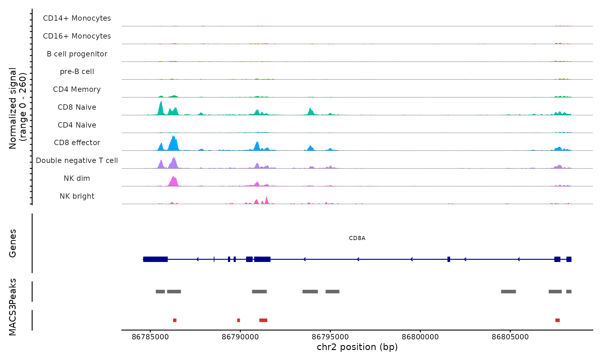
Session Info
## R version 4.5.0 (2025-04-11)
## Platform: x86_64-pc-linux-gnu
## Running under: Red Hat Enterprise Linux 8.10 (Ootpa)
##
## Matrix products: default
## BLAS:   /charonfs/home/users/astar/gis/stuartt/R-4.5.0/lib/libRblas.so
## LAPACK: /charonfs/home/users/astar/gis/stuartt/R-4.5.0/lib/libRlapack.so;  LAPACK version 3.12.1
##
## locale:
##  [1] LC_CTYPE=en_US.UTF-8       LC_NUMERIC=C
##  [3] LC_TIME=en_US.UTF-8        LC_COLLATE=en_US.UTF-8
##  [5] LC_MONETARY=en_US.UTF-8    LC_MESSAGES=en_US.UTF-8
##  [7] LC_PAPER=en_US.UTF-8       LC_NAME=C
##  [9] LC_ADDRESS=C               LC_TELEPHONE=C
## [11] LC_MEASUREMENT=en_US.UTF-8 LC_IDENTIFICATION=C
##
## time zone: Asia/Singapore
## tzcode source: system (glibc)
##
## attached base packages:
## [1] stats     graphics  grDevices utils     datasets  methods   base
##
## other attached packages:
## [1] future_1.70.0      Seurat_5.4.0       SeuratObject_5.3.0 sp_2.2-1
## [5] Signac_1.9999.0
##
## loaded via a namespace (and not attached):
##   [1] RColorBrewer_1.1-3          jsonlite_2.0.0
##   [3] magrittr_2.0.4              spatstat.utils_3.2-1
##   [5] farver_2.1.2                rmarkdown_2.30
##   [7] fs_1.6.7                    ragg_1.5.0
##   [9] vctrs_0.7.1                 ROCR_1.0-12
##  [11] spatstat.explore_3.7-0      Rsamtools_2.26.0
##  [13] RcppRoll_0.3.1              htmltools_0.5.9
##  [15] S4Arrays_1.10.1             SparseArray_1.10.8
##  [17] sass_0.4.10                 sctransform_0.4.3
##  [19] parallelly_1.46.1           KernSmooth_2.23-26
##  [21] bslib_0.10.0                htmlwidgets_1.6.4
##  [23] desc_1.4.3                  ica_1.0-3
##  [25] plyr_1.8.9                  plotly_4.12.0
##  [27] zoo_1.8-15                  cachem_1.1.0
##  [29] igraph_2.2.2                mime_0.13
##  [31] lifecycle_1.0.5             pkgconfig_2.0.3
##  [33] Matrix_1.7-4                R6_2.6.1
##  [35] fastmap_1.2.0               MatrixGenerics_1.22.0
##  [37] fitdistrplus_1.2-6          shiny_1.13.0
##  [39] digest_0.6.39               patchwork_1.3.2
##  [41] S4Vectors_0.48.0            tensor_1.5.1
##  [43] RSpectra_0.16-2             irlba_2.3.7
##  [45] textshaping_1.0.4           GenomicRanges_1.62.1
##  [47] labeling_0.4.3              progressr_0.18.0
##  [49] spatstat.sparse_3.1-0       polyclip_1.10-7
##  [51] httr_1.4.8                  abind_1.4-8
##  [53] compiler_4.5.0              withr_3.0.2
##  [55] S7_0.2.1                    BiocParallel_1.44.0
##  [57] fastDummies_1.7.5           MASS_7.3-65
##  [59] DelayedArray_0.36.0         tools_4.5.0
##  [61] lmtest_0.9-40               otel_0.2.0
##  [63] httpuv_1.6.16               future.apply_1.20.2
##  [65] goftest_1.2-3               glue_1.8.0
##  [67] InteractionSet_1.38.0       nlme_3.1-168
##  [69] promises_1.5.0              grid_4.5.0
##  [71] Rtsne_0.17                  cluster_2.1.8.2
##  [73] reshape2_1.4.5              generics_0.1.4
##  [75] spatstat.data_3.1-9         gtable_0.3.6
##  [77] tidyr_1.3.2                 data.table_1.18.2.1
##  [79] stringfish_0.18.0           XVector_0.50.0
##  [81] spatstat.geom_3.7-0         BiocGenerics_0.56.0
##  [83] RcppAnnoy_0.0.23            ggrepel_0.9.7
##  [85] RANN_2.6.2                  pillar_1.11.1
##  [87] stringr_1.6.0               spam_2.11-3
##  [89] RcppHNSW_0.6.0              later_1.4.8
##  [91] splines_4.5.0               dplyr_1.2.0
##  [93] lattice_0.22-9              deldir_2.0-4
##  [95] survival_3.8-6              tidyselect_1.2.1
##  [97] Biostrings_2.78.0           miniUI_0.1.2
##  [99] pbapply_1.7-4               knitr_1.51
## [101] gridExtra_2.3               IRanges_2.44.0
## [103] Seqinfo_1.0.0               SummarizedExperiment_1.40.0
## [105] scattermore_1.2             stats4_4.5.0
## [107] xfun_0.56                   Biobase_2.70.0
## [109] matrixStats_1.5.0           stringi_1.8.7
## [111] UCSC.utils_1.6.1            lazyeval_0.2.2
## [113] yaml_2.3.12                 evaluate_1.0.5
## [115] codetools_0.2-20            tibble_3.3.1
## [117] cli_3.6.5                   RcppParallel_5.1.11-1
## [119] uwot_0.2.4                  xtable_1.8-8
## [121] reticulate_1.45.0           systemfonts_1.3.2
## [123] jquerylib_0.1.4             dichromat_2.0-0.1
## [125] Rcpp_1.1.1                  GenomeInfoDb_1.46.2
## [127] spatstat.random_3.4-4       globals_0.19.1
## [129] png_0.1-9                   spatstat.univar_3.1-6
## [131] parallel_4.5.0              pkgdown_2.2.0
## [133] ggplot2_4.0.2               dotCall64_1.2
## [135] sparseMatrixStats_1.22.0    bitops_1.0-9
## [137] listenv_0.10.1              viridisLite_0.4.3
## [139] scales_1.4.0                ggridges_0.5.7
## [141] purrr_1.2.1                 crayon_1.5.3
## [143] rlang_1.1.7                 qs2_0.1.7
## [145] cowplot_1.2.0               fastmatch_1.1-8