Plot frequency of Tn5 insertion events for different groups of cells within given regions of the genome. Tracks are normalized using a per-group scaling factor computed as the number of cells in the group multiplied by the mean sequencing depth for that group of cells. This accounts for differences in number of cells and potential differences in sequencing depth between groups.
Usage
CoveragePlot(
  object,
  region,
  features = NULL,
  assay = NULL,
  split.assays = FALSE,
  assay.scale = "common",
  show.bulk = FALSE,
  expression.assay = "RNA",
  expression.slot = "data",
  annotation = TRUE,
  peaks = TRUE,
  peaks.group.by = NULL,
  ranges = NULL,
  ranges.group.by = NULL,
  ranges.title = "Ranges",
  region.highlight = NULL,
  links = "linkpeaks",
  tile = FALSE,
  tile.size = 100,
  tile.cells = 100,
  bigwig = NULL,
  bigwig.type = "coverage",
  bigwig.scale = "common",
  heights = NULL,
  group.by = NULL,
  split.by = NULL,
  window = 100,
  extend.upstream = 0,
  extend.downstream = 0,
  scale.factor = NULL,
  ymax = NULL,
  cells = NULL,
  idents = NULL,
  max.downsample = 3000,
  downsample.rate = 0.1,
  gwas = NULL,
  gwas.ld.file = NULL,
  gwas.ld.lead.snp = NULL,
  gwas.credset.file = NULL,
  gwas.credset.threshold = 0.01,
  variants = NULL,
  ...
)
Arguments
- object
A Seurat object
- region
A set of genomic coordinates to show. Can be a GRanges object, a string encoding a genomic position, a gene name, or a vector of strings describing the genomic coordinates or gene names to plot. If a gene name is supplied, annotations must be present in the assay.
- features
A vector of features present in another assay to plot alongside accessibility tracks (for example, gene names).
- assay
Name of the assay to plot. If a list of assays is provided, data from each assay will be shown overlaid on each track. The first assay in the list will define the assay used for gene annotations, links, and peaks (if shown). The order of assays given defines the plotting order.
- split.assays
When plotting data from multiple assays, display each assay as a separate track. If FALSE, data from different assays are overlaid on a single track with transparancy applied.
- assay.scale
Scaling to apply to data from different assays. Can be:
common: plot all assays on a common scale (default)
separate: plot each assay on a separate scale ranging from zero to the maximum value for that assay within the plotted region
- show.bulk
Include coverage track for all cells combined (pseudo-bulk). Note that this will plot the combined accessibility for all cells included in the plot (rather than all cells in the object).
- expression.assay
Name of the assay containing expression data to plot alongside accessibility tracks. Only needed if supplying
featuresargument.- expression.slot
Name of slot to pull expression data from. Only needed if supplying the
featuresargument.- annotation
Display gene annotations. Set to TRUE or FALSE to control whether genes models are displayed, or choose "transcript" to display all transcript isoforms, or "gene" to display gene models only (same as setting TRUE).
- peaks
Display peaks
- peaks.group.by
Grouping variable to color peaks by. Must be a variable present in the feature metadata. If NULL, do not color peaks by any variable.
- ranges
Additional genomic ranges to plot
- ranges.group.by
Grouping variable to color ranges by. Must be a variable present in the metadata stored in the
rangesgenomic ranges. If NULL, do not color by any variable.- ranges.title
Y-axis title for ranges track. Only relevant if
rangesparameter is set.- region.highlight
Region to highlight on the plot. Should be a GRanges object containing the coordinates to highlight. By default, regions will be highlighted in grey. To change the color of the highlighting, include a metadata column in the GRanges object named "color" containing the color to use for each region.
- links
Character vector containing the keys of link information present in the assay to display. Default is "linkpeaks" which is the default key for peak-gene links stored using the
LinkPeaks()function. IfNULL, links will not be displayed.- tile
Display per-cell fragment information in sliding windows. If plotting multi-assay data, only the first assay is shown in the tile plot.
- tile.size
Size of the sliding window for per-cell fragment tile plot
- tile.cells
Number of cells to display fragment information for in tile plot.
- bigwig
List of bigWig file paths to plot data from. Files can be remotely hosted. The name of each element in the list will determine the y-axis label given to the track.
- bigwig.type
Type of track to use for bigWig files ("line", "heatmap", or "coverage"). Should either be a single value, or a list of values giving the type for each individual track in the provided list of bigwig files.
- bigwig.scale
Same as
assay.scaleparameter, except for bigWig files when plotted withbigwig.type="coverage"- heights
Relative heights for each track (accessibility, gene annotations, peaks, links).
- group.by
Name of one or more metadata columns to group (color) the cells by. Default is the current cell identities
- split.by
A metadata variable to split the tracks by. For example, grouping by "celltype" and splitting by "batch" will create separate tracks for each combination of celltype and batch.
- window
Smoothing window size
- extend.upstream
Number of bases to extend the region upstream.
- extend.downstream
Number of bases to extend the region downstream.
- scale.factor
Scaling factor for track height. If NULL (default), use the median group scaling factor determined by total number of fragments sequences in each group.
- ymax
Maximum value for Y axis. Can be one of:
NULL: set to the highest value among all the tracks (default)qXX: clip the maximum value to the XX quantile (for example, q95 will set the maximum value to 95% of the maximum value in the data). This can help remove the effect of extreme values that may otherwise distort the scale.
numeric: manually define a Y-axis limit
- cells
Which cells to plot. Default all cells
- idents
Which identities to include in the plot. Default is all identities.
- max.downsample
Minimum number of positions kept when downsampling. Downsampling rate is adaptive to the window size, but this parameter will set the minimum possible number of positions to include so that plots do not become too sparse when the window size is small.
- downsample.rate
Fraction of positions to retain when downsampling. Retaining more positions can give a higher-resolution plot but can make the number of points large, resulting in larger file sizes when saving the plot and a longer period of time needed to draw the plot.
- gwas
GWAS summary statistics to display on the plot. Can be the path to a GWAS-SSF file on-disk or a dataframe in the GWAS-SSF format.
- gwas.ld.file
Path to LD data file for coloring GWAS points by r². Optional.
- gwas.ld.lead.snp
Lead SNP for LD calculations. Required if gwas.ld.file provided.
- gwas.credset.file
Path to fine-mapping credible sets file. Optional.
- gwas.credset.threshold
Posterior probability threshold for credible sets (default: 0.01)
- variants
Dataframe containing variants to display (see
VariantTrack())- ...
Additional arguments passed to
patchwork::wrap_plots()
Value
Returns a patchwork::patchwork() object
Details
Additional information can be layered on the coverage plot by setting several different options in the CoveragePlot function. This includes showing:
gene annotations
peak positions
additional genomic ranges
additional data stored in a bigWig file, which may be hosted remotely
gene or protein expression data alongside coverage tracks
peak-gene links
the position of individual sequenced fragments as a heatmap
data for multiple chromatin assays simultaneously
a pseudobulk for all cells combined
Examples
# \donttest{
fpath <- system.file("extdata", "fragments.tsv.gz", package = "Signac")
fragments <- CreateFragmentObject(
path = fpath,
cells = colnames(atac_small),
validate.fragments = FALSE
)
#> Computing hash
Fragments(atac_small) <- fragments
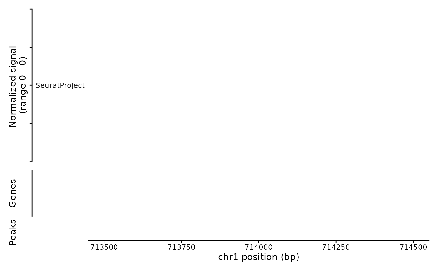
# Basic coverage plot
CoveragePlot(object = atac_small, region = c("chr1:713500-714500"))
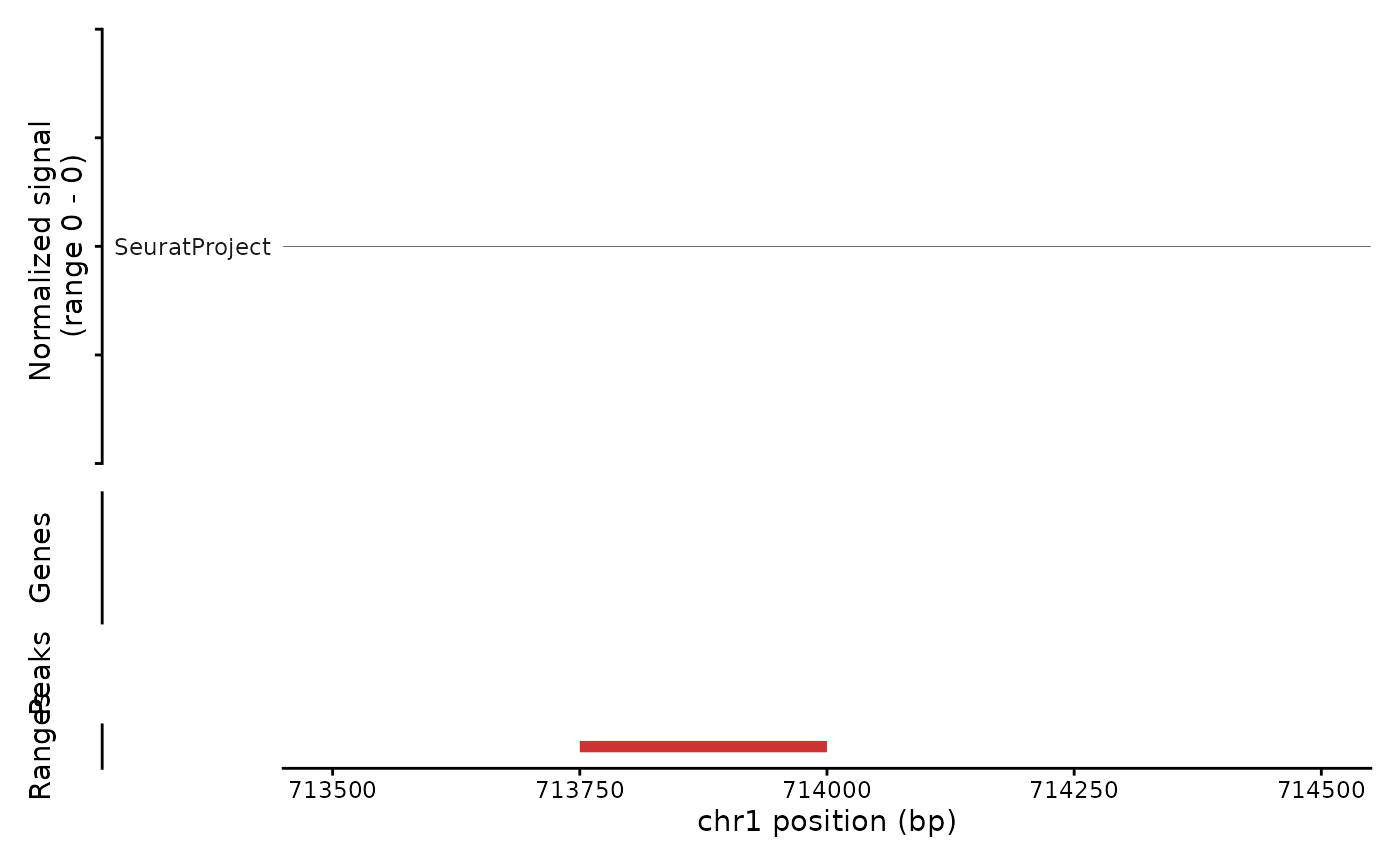
 # Show additional ranges
ranges.show <- GenomicRanges::GRanges("chr1:713750-714000")
CoveragePlot(
object = atac_small,
region = c("chr1:713500-714500"),
ranges = ranges.show
)
# Show additional ranges
ranges.show <- GenomicRanges::GRanges("chr1:713750-714000")
CoveragePlot(
object = atac_small,
region = c("chr1:713500-714500"),
ranges = ranges.show
)
 # Highlight region
CoveragePlot(
object = atac_small,
region = c("chr1:713500-714500"),
region.highlight = ranges.show
)
# Highlight region
CoveragePlot(
object = atac_small,
region = c("chr1:713500-714500"),
region.highlight = ranges.show
)
 # Change highlight color
ranges.show$color <- "orange"
CoveragePlot(
object = atac_small,
region = c("chr1:713500-714500"),
region.highlight = ranges.show
)
# Change highlight color
ranges.show$color <- "orange"
CoveragePlot(
object = atac_small,
region = c("chr1:713500-714500"),
region.highlight = ranges.show
)
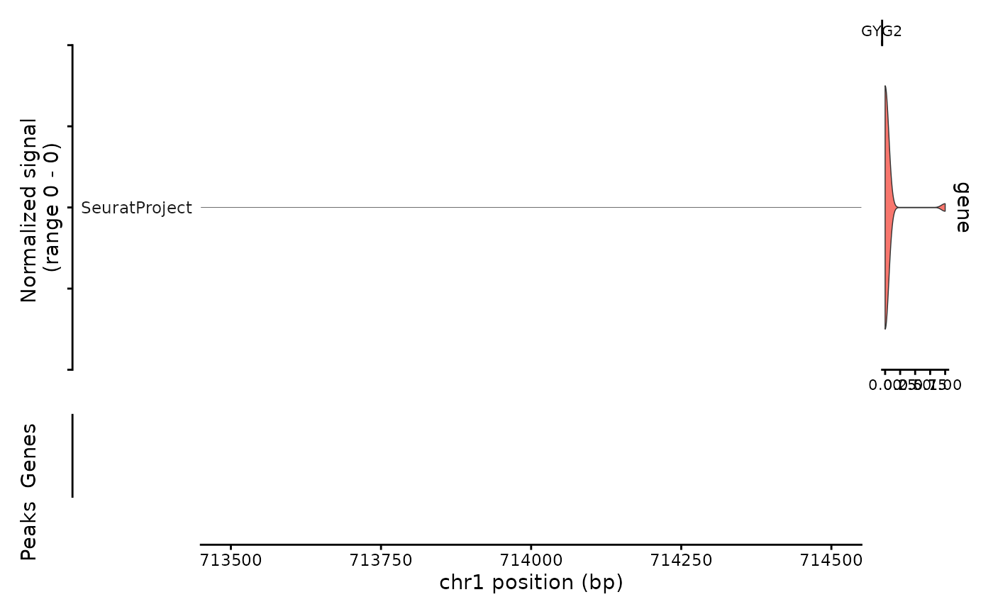
 # Show expression data
CoveragePlot(
object = atac_small,
region = c("chr1:713500-714500"),
features = "GYG2"
)
# Show expression data
CoveragePlot(
object = atac_small,
region = c("chr1:713500-714500"),
features = "GYG2"
)
 # }
# }