
Joint single-cell mitochondrial DNA genotyping and DNA accessibility analysis
Caleb Lareau and Tim Stuart
Compiled: July 30, 2026
Source:vignettes/mito.Rmd
mito.Rmd
library(Signac)
library(Seurat)
library(ggplot2)
library(ggrepel)
library(patchwork)
library(EnsDb.Hsapiens.v86)
In this vignette, we take a look at two different datasets containing both DNA accessibility measurements and mitochondrial mutation data in the same cells. One was sampled from a patient with a colorectal cancer (CRC) tumor, and the other is from a polyclonal TF1 cell line. This data was produced by Lareau and Ludwig et al. (2020), and you can read the original paper here: https://doi.org/10.1038/s41587-020-0645-6.
We have re-processed the original data mapping to the hg38 genome. These updated files, including mitochondrial variant data for the CRC and TF1 datasets, are available on Zenodo here: https://zenodo.org/records/19450459
Original sequencing reads and processed data mapped to hg19 for the these datasets are available on NCBI GEO here: https://www.ncbi.nlm.nih.gov/geo/query/acc.cgi?acc=GSE142745
View data download code
The required files can be downloaded by running the following lines in a shell:
Colorectal cancer dataset
To demonstrate combined analyses of mitochondrial DNA variants and accessible chromatin, we’ll walk through a vignette analyzing cells from a primary colorectal adenocarcinoma. The sample contains a mixture of malignant epithelial cells and tumor infiltrating immune cells.
Loading the DNA accessibility data
First we load the scATAC-seq data and create a Seurat object following the standard workflow for scATAC-seq data.
# load counts and metadata from cellranger-atac
counts <- Read10X_h5(filename = "crc/atac/crc_filtered_peak_bc_matrix.h5")

metadata <- read.csv(file = "crc/atac/crc_singlecell.csv",
                     header = TRUE,
                     row.names = 1)

# load gene annotations from Ensembl
annotations <- GetGRangesFromEnsDb(ensdb = EnsDb.Hsapiens.v86)

# change to UCSC style since the data was mapped to hg38 UCSC
seqlevels(annotations) <- paste0("chr", seqlevels(annotations))
genome(annotations) <- "hg38"

# create object
crc_assay <- CreateGRangesAssay(
  counts = counts,
  annotation = annotations,
  min.cells = 10,
  fragments = "crc/atac/crc_fragments.tsv.gz"
)

crc <- CreateSeuratObject(
  counts = crc_assay,
  assay = "peaks",
  meta.data = metadata
)

crc[["peaks"]]
## GRangesAssay data with 104502 features for 3530 cells
## Variable features: 0
## Annotation present: TRUE
## Fragment files: 1
## Motifs present: FALSE
## Links present: 0
## Region aggregation matrices: 0Quality control
We can compute the standard quality control metrics for scATAC-seq and filter out low-quality cells based on these metrics. Additionally, we import the mean mitochondrial depth per cell (total mt base counts/length of mtDNA contig) from mgatk to filter out cells with low mtDNA depth.
# Augment QC metrics that were computed by cellranger-atac
crc$pct_reads_in_peaks <- crc$peak_region_fragments / crc$passed_filters * 100

# compute TSS enrichment score and nucleosome banding pattern
crc <- ATACqc(crc)

# Import mtDNA depth & add to metadata
mito.depth <- read.delim("crc/mgatk/mgatk_crc.depthTable.txt",
                         header = FALSE,
                         row.names = 1,
                         col.names = c("cell","mtDNA_depth"))

crc <- AddMetaData(object = crc, metadata = mito.depth)
# visualize QC metrics for each cell
VlnPlot(crc,
        c("TSS_enrichment", "nCount_peaks", "Nucleosome_signal", "Mito_fraction", "mtDNA_depth"),
        pt.size = 0.1,
        ncol = 5) + scale_y_log10()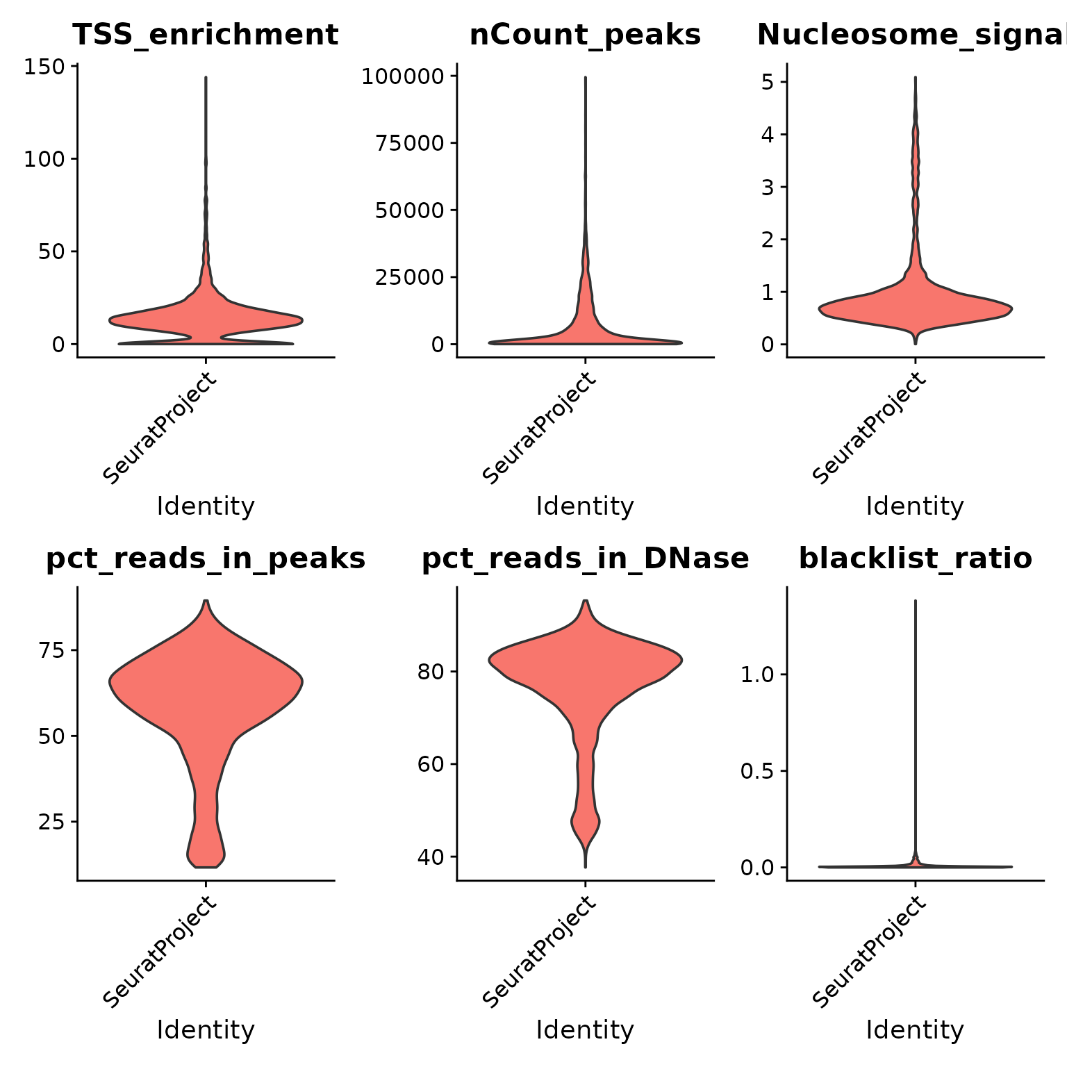
# remove low-quality cells
crc <- subset(
  x = crc,
  subset = nCount_peaks > 1000 &
    nCount_peaks < 50000 &
    TSS_enrichment > 3 &
    Nucleosome_signal < 4 &
    mtDNA_depth >=10
)
crc
## An object of class Seurat
## 104502 features across 1528 samples within 1 assay
## Active assay: peaks (104502 features, 0 variable features)
## 1 layer present: countsDimension reduction and clustering
Next we can run a standard dimension reduction and clustering workflow using the scATAC-seq data to identify cell clusters.
crc <- RunTFIDF(crc)
crc <- FindTopFeatures(crc, min.cutoff = 10)
crc <- RunSVD(crc)
crc <- RunUMAP(crc, reduction = "lsi", dims = 2:50)
crc <- FindNeighbors(crc, reduction = "lsi", dims = 2:50)
crc <- FindClusters(crc, resolution = 0.5, algorithm = 3)
## Modularity Optimizer version 1.3.0 by Ludo Waltman and Nees Jan van Eck
##
## Number of nodes: 1528
## Number of edges: 60096
##
## Running smart local moving algorithm...
## Maximum modularity in 10 random starts: 0.8284
## Number of communities: 7
## Elapsed time: 0 seconds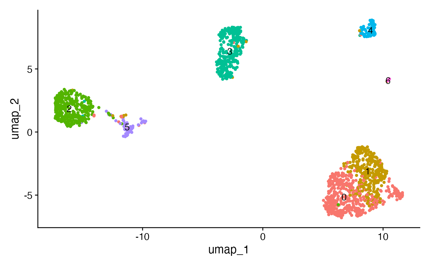
Generate gene scores
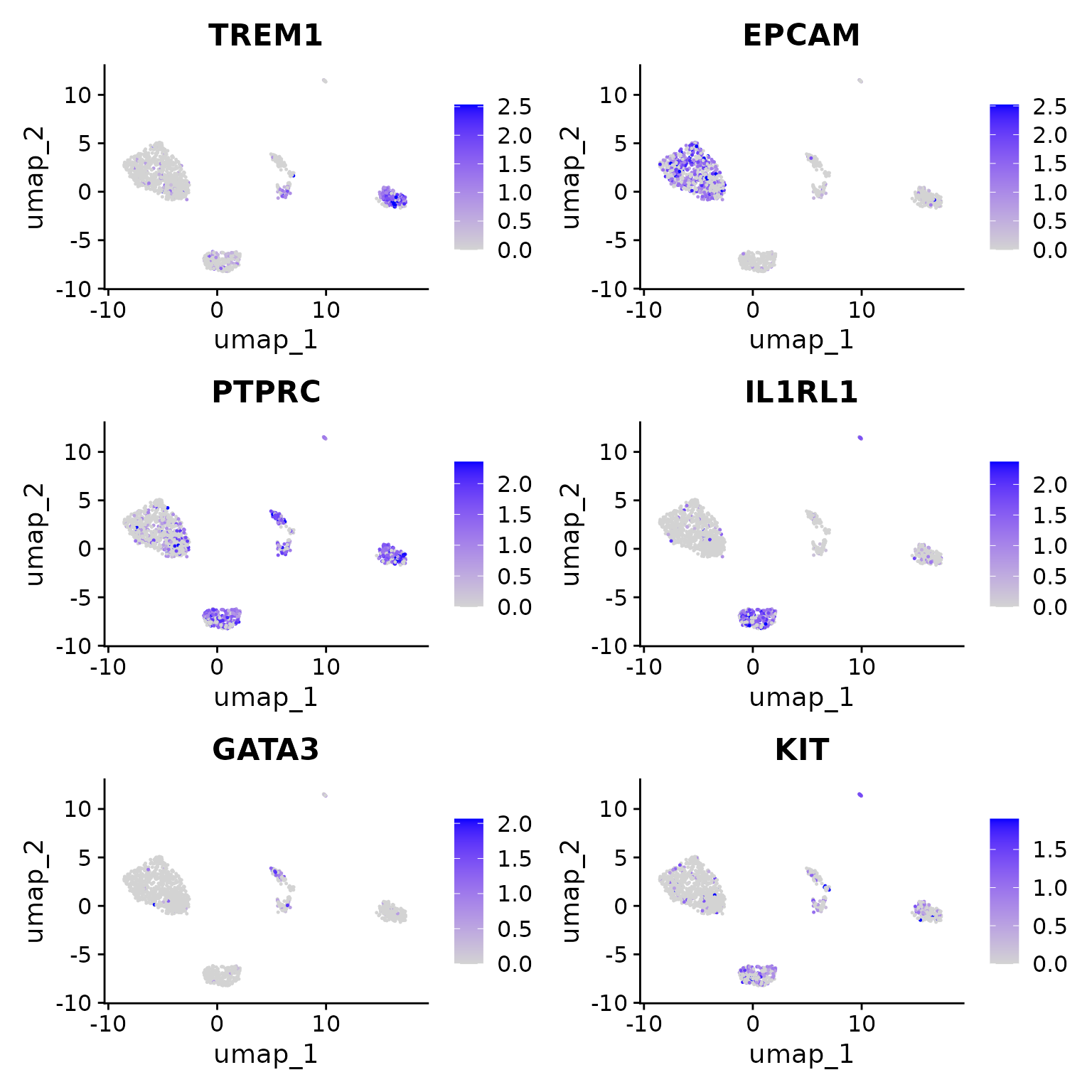
To help interpret these clusters of cells, and assign a cell type label, we’ll estimate gene activities by summing the DNA accessibility in the gene body and promoter region.
# compute gene accessibility
gene.activities <- GeneActivity(crc)

# add to the Seurat object as a new assay
rownames(gene.activities) <- make.unique(rownames(gene.activities))
crc[["RNA"]] <- CreateAssay5Object(counts = gene.activities)

crc <- NormalizeData(object = crc, assay = "RNA")
Visualize interesting gene activity scores
We note the following markers for different cell types in the CRC dataset:
- EPCAM is a marker for epithelial cells
- TREM1 is a myeloid marker
- PTPRC = CD45 is a pan-immune cell marker
- IL1RL1 is a basophil marker
- GATA3 is a Tcell maker
DefaultAssay(crc) <- "RNA"

FeaturePlot(
  object = crc,
  features = c("TREM1", "EPCAM", "PTPRC", "IL1RL1", "GATA3", "KIT"),
  pt.size = 0.1,
  max.cutoff = "q95",
  ncol = 2
)
One of the myeloid clusters has a lower percentage of fragments in peaks, as well as a lower overall mitochondrial sequencing depth and a different nucleosome banding pattern.
p1 <- FeatureScatter(crc, "mtDNA_depth", "pct_reads_in_peaks") + ggtitle("") + scale_x_log10()
p2 <- FeatureScatter(crc, "mtDNA_depth", "Nucleosome_signal") + ggtitle("") + scale_x_log10()

p1 + p2 + plot_layout(guides = "collect")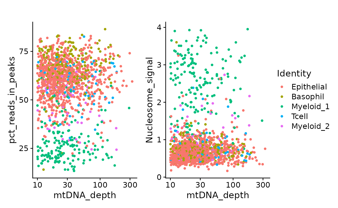
We can see that most of the low FRIP cells were the myeloid cluster. This is most likely an intra-tumor granulocyte that has relatively poor accessible chromatin enrichment. Similarly, the unusual nuclear chromatin packaging of this cell type yields slightly reduced mtDNA coverage compared to the other myeloid cluster.
Mitochondrial variant analysis
We now import the mitochondrial variant data identified by two tools - mgatk or MQuad. The former performs genotyping of mtDNA variants & identifies high confidence variants using strand correlation & variance mean ratio metrics. The latter takes in genotyped mitochondrial DNA data and identifies informative variants using a binomial mixture model to assess heteroplasmy. Both tools provide a list of useful mitochondrial variants that provide clonal information, as we will see below.
We observe significant overlap of mitochondrial variants identified between both tools, with differences due to the their approaches in classifying informativeness.
mgatk
In this tab, we load mitochondrial DNA variant data that was
quantified using mgatk.
Load mgatk mitochondrial DNA variant data
The ReadMGATK()function in Signac allows the output to
be read directly into R in a convenient format for downstream analysis
with Signac. ReadMGATK() returns a list containing the
mitochondrial allele counts at each position & 2 dataframes
containing the depth and reference allele. Here, we load the data and
add the counts to the Seurat object as a new assay.
# load mgatk output
mgatk.data <- ReadMGATK(dir = "crc/mgatk")

# create an assay
mgatk <- CreateAssay5Object(counts = mgatk.data$counts)

# Subset to cells present in the scATAC-seq assay
mgatk <- subset(mgatk, cells = Cells(crc))

# add assay and metadata to the seurat object
crc[["mgatk"]] <- mgatk
mgatk informative mtDNA variants
Next, we can identify sites in the mitochondrial genome that vary across cells, and cluster the cells into clonotypes based on the frequency of these variants in the cells. Signac utilizes the principles established in the original mtscATAC-seq work of identifying high-quality variants.
variable.sites <- IdentifyVariants(crc,
                                   assay = "mgatk",
                                   refallele = mgatk.data$refallele)
VariantPlot(variants = variable.sites)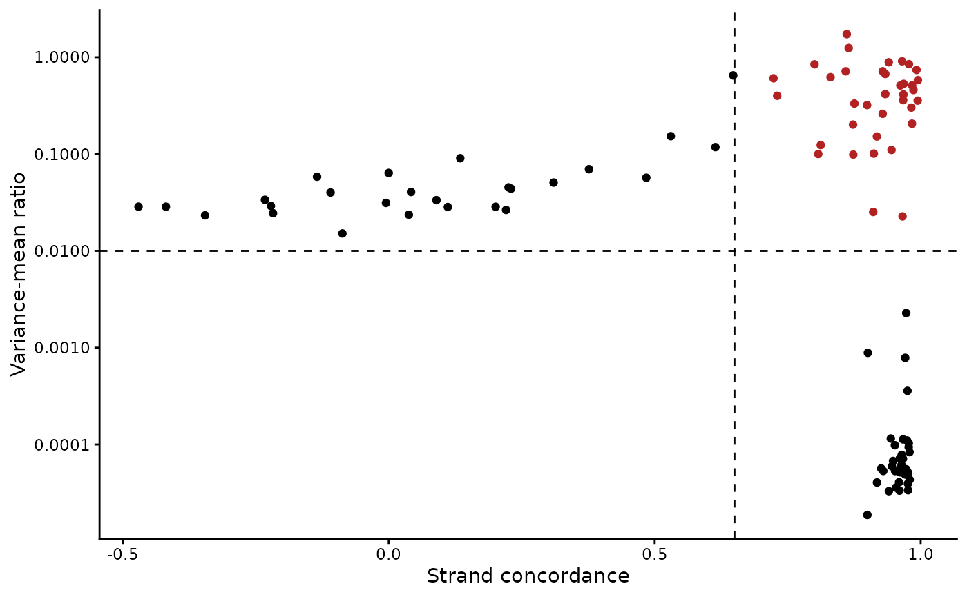
The plot above clearly shows a group of variants with a higher VMR and strand concordance. In principle, a high strand concordance reduces the likelihood of the allele frequency being driven by sequencing error (which predominately occurs on one but not the other strand. This is due to the preceding nucleotide content and a common error in mtDNA genotyping). On the other hand, variants that have a high VMR are more likely to be clonal variants as the alternate alleles tend to aggregate in certain cells rather than be equivalently dispersed about all cells, which would be indicative of some other artifact.
We note that variants that have a very low VMR and and very high strand concordance are homoplasmic variants for this sample. While these may be interesting in some settings (e.g. donor demultiplexing), for inferring subclones, these are not particularly useful.
Based on these thresholds, we can filter out a set of informative mitochondrial variants that differ across the cells.
# Establish a filtered data frame of variants based on this processing
high.conf <- subset(
  variable.sites,
  subset = n_cells_conf_detected >= 5 &
    strand_correlation >= 0.65 &
    vmr > 0.01
)

high.conf[, c(1, 2, 5)]
## position nucleotide mean
## 1227G>A 1227 G>A 0.0081258
## 3244G>A 3244 G>A 0.0011659
## 6081G>A 6081 G>A 0.0028495
## 9804G>A 9804 G>A 0.0031600
## 12889G>A 12889 G>A 0.0214799
## 9728C>T 9728 C>T 0.0131214
## 16147C>T 16147 C>T 0.5967952
## 824T>C 824 T>C 0.0057065
## 2285T>C 2285 T>C 0.0055697
## 9840T>C 9840 T>C 0.0020045
## 16093T>C 16093 T>C 0.0073883
## 2623A>G 2623 A>G 0.0016689A few things stand out. First, 9 out of the 12 variants occur at less than 1% allele frequency in the population. However, 16147C>T is present at about 59.7%. We’ll see that this is a clonal variant marking the epithelial cells. Additionally, all of the called variants are transitions (A - G or C - T) rather than transversion mutations (A - T or C - G). This fits what we know about how these mutations arise in the mitochondrial genome.
Depending on your analytical question, these thresholds can be adjusted to identify variants that are more prevalent in other cells.
Compute allele frequency of informative mgatk variants for each cell
We currently have information for each strand stored in the
mgatk assay to allow strand concordance to be assessed. Now
that we have our set of high-confidence informative variants, we can
create a new assay containing strand-collapsed allele frequency counts
for each cell for these variants using the AlleleFreq()
function.
crc <- AlleleFreq(
  object = crc,
  variants = high.conf$variant,
  assay = "mgatk",
  new.assay.name = "mgatk_af"
)
crc[["mgatk_af"]]
## Assay data with 12 features for 1528 cells
## First 10 features:
## 1227G>A, 3244G>A, 6081G>A, 9804G>A, 12889G>A, 9728C>T, 16147C>T,
## 824T>C, 2285T>C, 9840T>CVisualize informative mgatk variants
Now that the allele frequencies are stored as an additional assay, we
can use the standard functions in Seurat to visualize how these allele
frequencies are distributed across the cells. Here we visualize a subset
of the variants identified by both mgatk and
MQuad using FeaturePlot().
DefaultAssay(crc) <- "mgatk_af"
alleles.view <- c("12889G>A", "16147C>T",
                  "9728C>T", "9804G>A")
FeaturePlot(
  object = crc,
  features = alleles.view,
  order = TRUE,
  cols = c("grey", "darkred"),
  ncol = 4
) & NoLegend()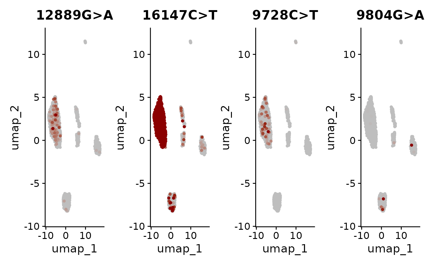
We also explore all informative mtDNA variants identified by
mgatk using DoHeatmap() to plot the allele
frequencies across all cells.
DoHeatmap(crc, features = sort(rownames(crc)), slot = "data", disp.max = 1) +
  scale_fill_viridis_c()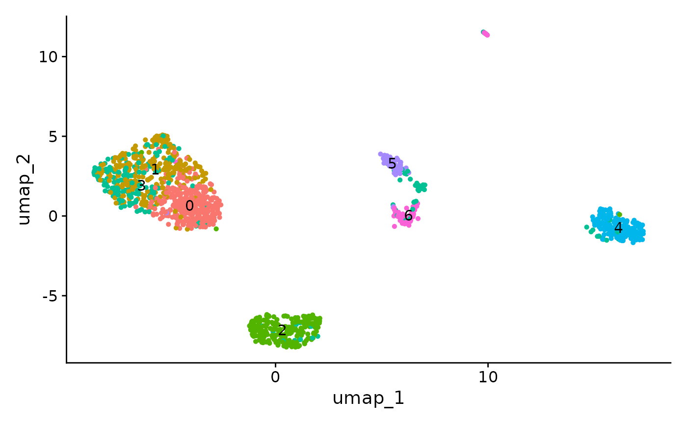
Here, we can see a few interesting patterns for the selected variants. 16147C>T is present in essentially all epithelial cells and almost exclusively in epithelial cells (the edge cases where this isn’t true are also cases where the UMAP and clustering don’t full agree). It is at 100% allele frequency– strongly suggestive of whatever cell of origin of this tumor had the mutation at 100% and then expanded. We then see at least 3 variants 1227G>A, 12889G>A, and 9728C>T that are mostly present specifically in the epithelial cells that define subclones. Other variants including 16093T>C, 9804G>A, and 824T>C are found specifically in immune cell populations, suggesting that these arose from a common hematopoetic progenitor cell (probably in the bone marrow).
MQuad
In this tab, we explore mitochondrial variants identified to be
clonally informative by MQuad. Bi-allelic genotyping of the
chrM DNA was performed using cellsnp-lite,
using the same reference as was used in mgatk (rCRS).
Load MQuad mitochondrial variant data
We load the AD (alternate allele depth) & DP (sum of alternate +
reference allele depth) sparse matrices for informative variants
identified by MQuad using the ReadMQuad
function. We will add the AD counts to the mquad assay, and
add the DP counts as another layer in the assay. These matrices will
then be used to calculate the allele frequency of the informative
variants per cell.
# load MQuad data
mquad.data <- ReadMQuad(dir = "crc/mquad",
                        cb = "crc/mquad/mquad_crc_cellSNP.samples.tsv")

# create an assay with AD counts of filtered cells
passed_cells <- as.vector(colnames(crc))
mquad <- CreateAssay5Object(counts = mquad.data$AD_matrix[,passed_cells])

# Add assay & add DP as layer
crc[["mquad"]] <- mquad
crc[["mquad"]]$DP <- mquad.data$DP_matrix[,passed_cells]
Compute allele frequency of informative MQuad variants for each cell
We compute the allele frequency & add to data slot of the
mquad assay. Note that there will be some 0 values in the
DP matrix, as some variants may not be detected in some cells. This will
result in some NA values in the allele frequency. We set these values to
0 in the data slot to facilitate downstream analysis. This will however
erase the biological significance between 0 (all ref) & NA (not
detected), and thus should be used with caution.
# compute VAF
mquad_vaf <- crc[["mquad"]]$counts / crc[["mquad"]]$DP
crc[["mquad"]]$data <- mquad_vaf

# Set NAs in VAF data to 0 (assuming not too many 0s)
crc[["mquad"]]$data[is.na(crc[["mquad"]]$data)] <- 0
Visualize informative MQuad variants
We can now visualize the subset of the variants identified by both
mgatk & MQuad using FeaturePlot().
DefaultAssay(crc) <- "mquad"
alleles.view <- c("12889G>A", "16147C>T",
                  "9728C>T", "9804G>A")
FeaturePlot(
  object = crc,
  features = alleles.view,
  order = TRUE,
  cols = c("grey", "darkred"),
  ncol = 4
) & NoLegend()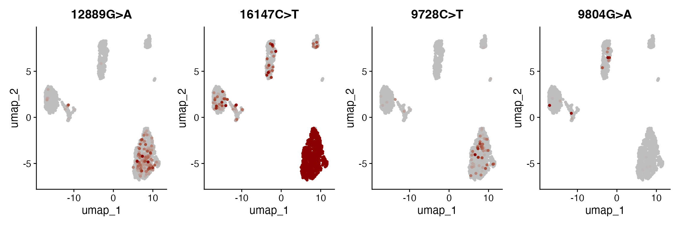
We also explore all informative mtDNA variants identified by
MQuad using DoHeatmap() to plot the allele
frequencies across all cells.
DoHeatmap(crc, features = sort(rownames(crc)), slot = "data", disp.max = 1) +
  scale_fill_viridis_c()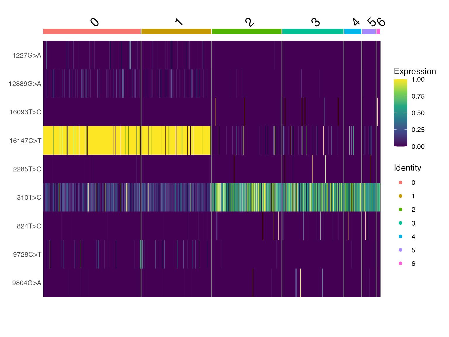
Investigate overlap between mgatk & MQuad variants
From the mgatk and MQuad heatmaps, the
detected mitochondrial variants mostly overlaps. We investigate the
overlapping and distinct variants further using an Euler diagram.
library(eulerr)

# list of variants by each tool
mgatk_variants <- high.conf$variant
mquad_variants <- rownames(mquad_vaf)

# plot Euler diagram
fit <- euler(list(mgatk = mgatk_variants, mquad = mquad_variants))
plot(fit, quantities = TRUE)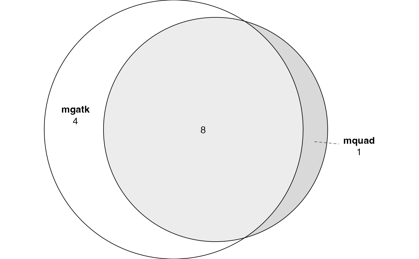
A total of 8 variants were commonly identified by mgatk
and MQuad. MQuad identified 1 unique
mitochondrial variant, while mgatk identified 4 other
unique variants that did not pass the BIC threshold in MQuad.
MQuad-specific variants
We now investigate the distinct variants by plotting them with
FeaturePlot().
# get distinct MQuad variants
mquad_unique <- setdiff(mquad_variants, mgatk_variants)

DefaultAssay(crc) <- "mquad"
FeaturePlot(
  object = crc,
  features = mquad_unique,
  order = TRUE,
  cols = c("grey", "darkred")
) & NoLegend()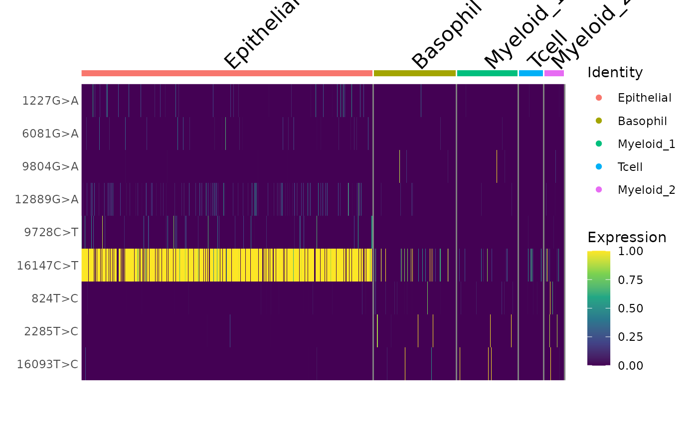
We can also visualize the distinct variants identified by MQuad on
the VariantPlot() to see where they are in the VMR-strand
concordance space.
p4 <- VariantPlot(variable.sites)

p4$data$highlight <- p4$data$variant %in% mquad_unique

p4 +
  geom_point(aes(color = highlight)) +
  scale_color_manual(values = c("grey", "blue")) +
  geom_text_repel(
    data = subset(p4$data, variant %in% mquad_unique),
    aes(label = variant),
    color = "blue"
  )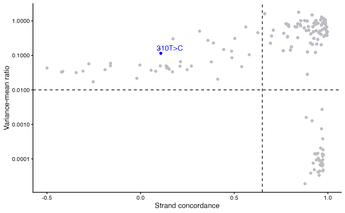
From the plot, the variant 310T>C was filtered out from mgatk as it did not pass the strand concordance test.
mgatk-specific variants
We next investigate mgatk distinct variants by plotting them with
FeaturePlot().
# get distinct mgatk variants
mgatk_unique <- setdiff(mgatk_variants, mquad_variants)

DefaultAssay(crc) <- "mgatk_af"
FeaturePlot(
  object = crc,
  features = mgatk_unique,
  order = TRUE,
  cols = c("grey", "darkred"),
  ncol = 4
) & NoLegend()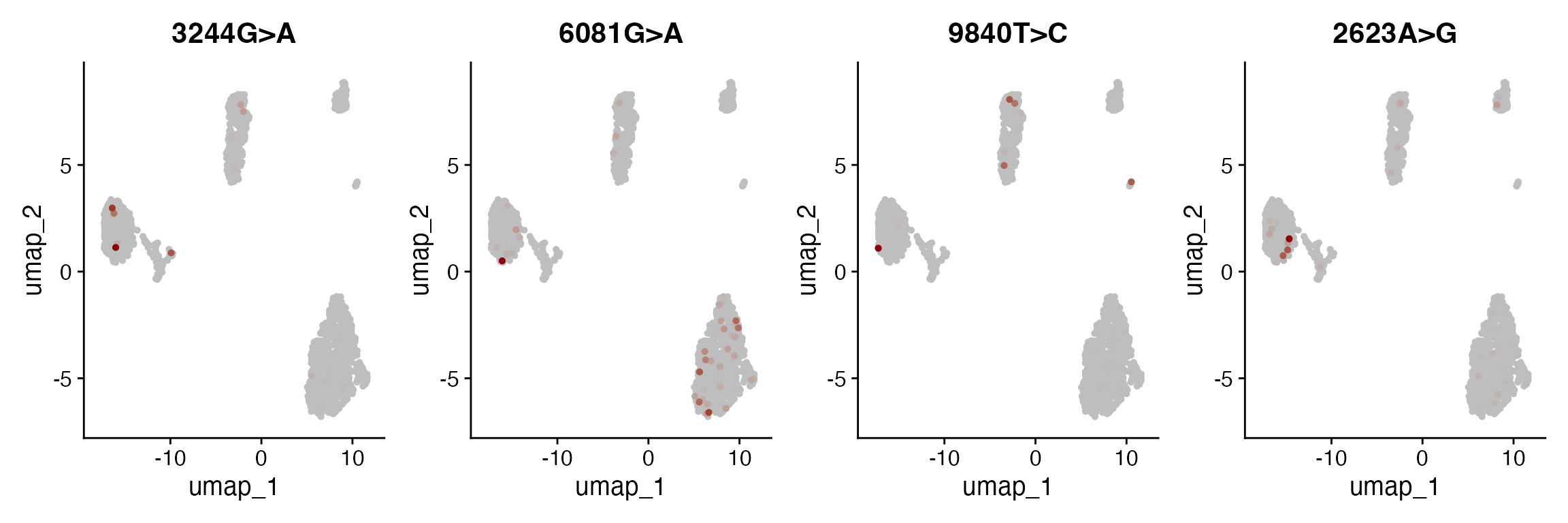
The above variants were filtered out by MQuad as they did not pass the cutoff in ΔBIC (Bayesian Information Criterion), and thus were not thought to be clonally informative.
Overall, both mitochondrial variant tools show high concordance, and either tool can be used for clonal analysis.
TF1 cell line dataset
Next we’ll demonstrate a similar workflow to identify cell clones in a different dataset, this time generated from a TF1 cell line. This dataset contains more clones present at a higher proportion, based on the experimental design.
We’ll demonstrate how to identify groups of related cells (clones) by clustering the allele frequency data and how to relate these clonal groups to accessibility differences utilizing the multimodal capabilities of Signac.
View data download code
To download the data from Zenodo run the following in a shell:
Loading the DNA accessibility data
As the data was generated from mixed cell lines (TF1 & GM11906), we subset the TF1-barcodes out from the peak matrix.
# load counts and metadata from cellranger-atac
counts <- Read10X_h5(filename = "tf1/atac/tf1_filtered_peak_bc_matrix.h5")

metadata <- read.csv(
  file = "tf1/atac/tf1_singlecell.csv",
  header = TRUE,
  row.names = 1
)

# create object
tf1_assay <- CreateGRangesAssay(
  counts = counts,
  annotation = annotations,
  min.cells = 10,
  fragments = "tf1/atac/tf1_fragments.tsv.gz"
)

tf1 <- CreateSeuratObject(
  counts = tf1_assay,
  assay = "peaks",
  meta.data = metadata
)

# Subset TF1 barcodes out
tf1_bc <- read.delim("tf1/atac/tf1_barcodes.tsv",
                     sep = '\t',
                     header = FALSE)

tf1 <- subset(tf1, cells = tf1_bc[,1])
tf1[["peaks"]]
## GRangesAssay data with 188266 features for 435 cells
## Variable features: 0
## Annotation present: TRUE
## Fragment files: 1
## Motifs present: FALSE
## Links present: 0
## Region aggregation matrices: 0Quality control
Compute the standard quality control metrics for scATAC-seq and filter out low-quality cells based on these metrics. We also import the mean mitochondrial depth per cell (total mt base counts/length of mtDNA contig) from mgatk to filter out cells with low mtDNA depth.
DefaultAssay(tf1) <- "peaks"

# compute TSS enrichment score and nucleosome banding pattern
tf1 <- ATACqc(object = tf1)

# Import mtDNA depth & add to metadata
mito.depth <- read.delim("tf1/mgatk/mgatk_tf1_1.depthTable.txt",
                         header = FALSE,
                         row.names = 1,
                         col.names = c("cell","mtDNA_depth"))

tf1 <- AddMetaData(object = tf1, metadata = mito.depth)
VlnPlot(tf1,
        c("TSS_enrichment", "nCount_peaks", "Nucleosome_signal","Mito_fraction", "mtDNA_depth"),
        pt.size = 0.1,
        ncol = 5) + scale_y_log10()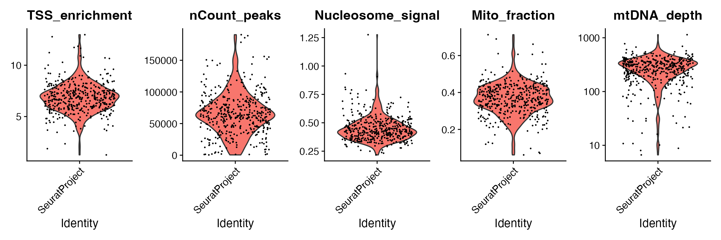
tf1 <- subset(
  x = tf1,
  subset = nCount_peaks > 500 &
    Nucleosome_signal < 1 &
    TSS_enrichment > 3 &
    mtDNA_depth >=10
)
tf1
## An object of class Seurat
## 188266 features across 427 samples within 1 assay
## Active assay: peaks (188266 features, 0 variable features)
## 1 layer present: countsMitochondrial variant analysis
Similarly, we analyze mitochondrial variants identified by
mgatk and MQuad in the TF1 dataset.
mgatk
In this tab, we load mitochondrial DNA variant data that was
quantified using mgatk.
Load mgatk mitochondrial DNA variant data
We load mgatk data using ReadMGATK()
function.
# read mgatk data
mgatk.data <- ReadMGATK(dir = "tf1/mgatk")
## Reading allele counts## Reading metadata## Building matrices
mgatk <- CreateAssayObject(counts = mgatk.data$counts)

# Subset to cells present in the scATAC-seq assay
mgatk <- subset(mgatk, cells = Cells(tf1))

# add assay and metadata to the seurat object
tf1[["mgatk"]] <- mgatk
mgatk informative mtDNA variants
Plot the VMR-strand concordance plot & identify high-confidence variants.
DefaultAssay(tf1) <- "mgatk"
variants <- IdentifyVariants(tf1, refallele = mgatk.data$refallele)
## Computing total coverage per base## Processing A## Processing T## Processing C## Processing G
VariantPlot(variants)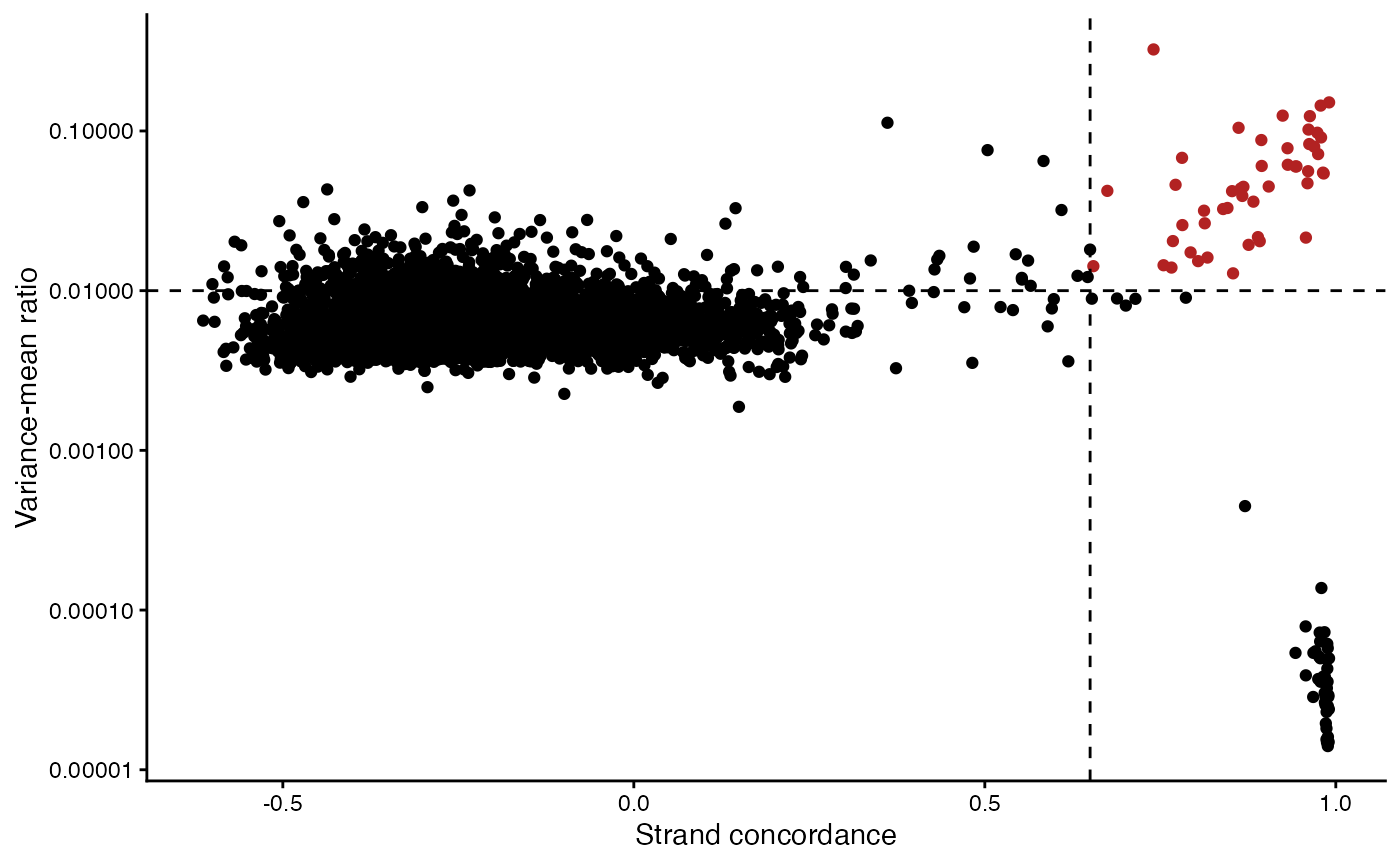
high.conf <- subset(
  variants,
  subset = n_cells_conf_detected >= 5 &
    strand_correlation >= 0.65 &
    vmr > 0.01
)
Calculate allele frequencies of the high confidence subset variants.
tf1 <- AlleleFreq(tf1,
                  variants = high.conf$variant,
                  assay = "mgatk",
                  new.assay.name = "mgatk_af")
tf1[["mgatk_af"]]
## Assay data with 40 features for 427 cells
## First 10 features:
## 627G>A, 709G>A, 1793G>A, 1888G>A, 2002G>A, 2573G>A, 2643G>A, 2954C>A,
## 3901G>A, 4037G>AIdentification of mgatk clones
Now that we’ve identified a set of variable alleles, we can cluster
the cells based on the frequency of each of these alleles using the
FindClonotypes() function.
DefaultAssay(tf1) <- "mgatk_af"
tf1 <- FindClonotypes(tf1)
## Modularity Optimizer version 1.3.0 by Ludo Waltman and Nees Jan van Eck
##
## Number of nodes: 427
## Number of edges: 6845
##
## Running smart local moving algorithm...
## Maximum modularity in 10 random starts: 0.8305
## Number of communities: 10
## Elapsed time: 0 seconds##
## 9 8 7 6 5 4 3 2 1 0
## 7 9 12 14 20 53 58 62 67 125Here we see that the clonal clustering has identified 9 different
clones in the TF1 dataset. We can further visualize the frequency of
alleles in these clones using DoHeatmap(). The
FindClonotypes() function also performs hierarchical
clustering on both the clonotypes and the alleles, and sets the factor
levels for the clonotypes based on the hierarchical clustering order,
and the order of variable features based on the hierarchical feature
clustering. This allows us to get a decent ordering of both features and
clones automatically:
DoHeatmap(tf1, features = VariableFeatures(tf1), slot = "data", disp.max = 0.3) +
  scale_fill_viridis_c()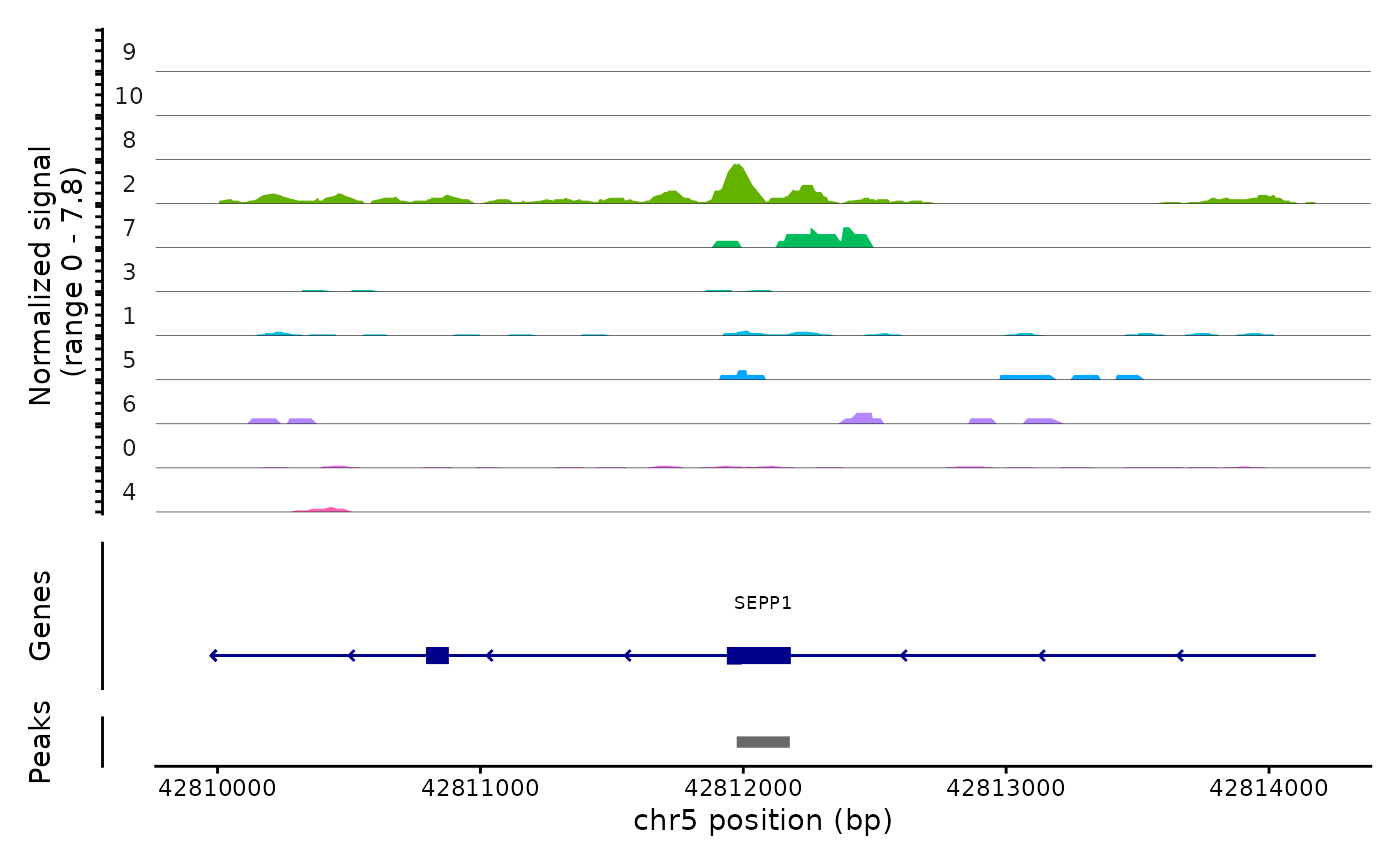
MQuad
In this tab, we load mitochondrial DNA variant data that was
quantified using MQuad.
Load MQuad mitochondrial DNA variant data
Import the AD & DP matrices using the ReadMQuad()
function.
mquad.data <- ReadMQuad(dir = "tf1/mquad",
                        cb = "tf1/mquad/tf1_mquad_cellSNP.samples.tsv")

# create an assay with AD counts of filtered cells
passed_cells <- as.vector(colnames(tf1))
mquad <- CreateAssay5Object(counts = mquad.data$AD_matrix[,passed_cells])

# Add assay & add DP as layer
tf1[["mquad"]] <- mquad
tf1[["mquad"]]$DP <- mquad.data$DP_matrix[,passed_cells]
Compute MQuad VAF & add to data slot of mquad assay.
# compute VAF
mquad_vaf <- tf1[["mquad"]]$counts / tf1[["mquad"]]$DP
tf1[["mquad"]]$data <- mquad_vaf

# Check number of 0 counts in DP matrix
sum(mquad.data$DP_matrix[,passed_cells] == 0)
## [1] 0## [1] 0
# Set NAs in VAF to 0
tf1[["mquad"]]$data[is.na(tf1[["mquad"]]$data)] <- 0
Identification of MQuad clones
We perform clonotype clustering using the identified MQuad variants.
DefaultAssay(tf1) <- "mquad"
tf1 <- FindClonotypes(tf1, assay = "mquad")
## Modularity Optimizer version 1.3.0 by Ludo Waltman and Nees Jan van Eck
##
## Number of nodes: 427
## Number of edges: 7134
##
## Running smart local moving algorithm...
## Maximum modularity in 10 random starts: 0.8363
## Number of communities: 10
## Elapsed time: 0 seconds##
## 9 7 8 6 5 4 3 2 1 0
## 9 11 11 14 19 53 56 62 68 124
DoHeatmap(tf1, features = VariableFeatures(tf1), slot = "data", disp.max = 0.3) +
  scale_fill_viridis_c()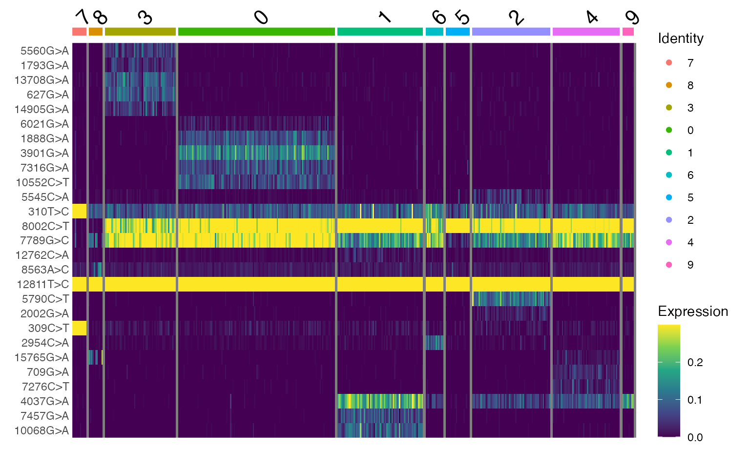
Investigate overlap between mgatk & MQuad variants
We investigate the common and unique variants identified using an Euler diagram.
# list of variants by each tool
mgatk_variants <- high.conf$variant
mquad_variants <- rownames(mquad_vaf)

# plot Euler diagram
fit <- euler(list(mgatk = mgatk_variants, mquad = mquad_variants))
plot(fit, quantities = TRUE)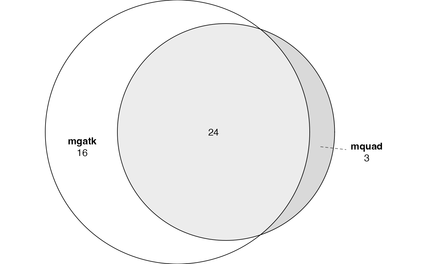
Again, we observe a significant subset of variants that are commonly identified between the 2 tools. Generally, we observe that MQuad results in a smaller subset of variants, likely due to stricter filtering criteria.
Session Info
## R version 4.5.1 (2025-06-13)
## Platform: aarch64-apple-darwin20
## Running under: macOS Tahoe 26.5.2
##
## Matrix products: default
## BLAS:   /Library/Frameworks/R.framework/Versions/4.5-arm64/Resources/lib/libRblas.0.dylib
## LAPACK: /Library/Frameworks/R.framework/Versions/4.5-arm64/Resources/lib/libRlapack.dylib;  LAPACK version 3.12.1
##
## locale:
## [1] en_US.UTF-8/en_US.UTF-8/en_US.UTF-8/C/en_US.UTF-8/en_US.UTF-8
##
## time zone: Australia/Perth
## tzcode source: internal
##
## attached base packages:
## [1] stats4    stats     graphics  grDevices utils     datasets  methods
## [8] base
##
## other attached packages:
##  [1] eulerr_8.1.0              future_1.75.0
##  [3] EnsDb.Hsapiens.v86_2.99.0 ensembldb_2.34.0
##  [5] AnnotationFilter_1.34.0   GenomicFeatures_1.62.0
##  [7] AnnotationDbi_1.72.0      Biobase_2.70.0
##  [9] GenomicRanges_1.62.1      Seqinfo_1.0.0
## [11] IRanges_2.44.0            S4Vectors_0.48.1
## [13] BiocGenerics_0.56.0       generics_0.1.4
## [15] patchwork_1.3.2           ggrepel_0.9.8
## [17] ggplot2_4.0.3             Seurat_5.5.1
## [19] SeuratObject_5.4.0        sp_2.2-3
## [21] Signac_1.9999.6
##
## loaded via a namespace (and not attached):
##   [1] fs_2.1.0                    ProtGenerics_1.42.0
##   [3] matrixStats_1.5.0           spatstat.sparse_3.2-0
##   [5] bitops_1.0-9                httr_1.4.8
##   [7] RColorBrewer_1.1-3          InteractionSet_1.38.0
##   [9] tools_4.5.1                 sctransform_0.4.3
##  [11] backports_1.5.1             R6_2.6.1
##  [13] lazyeval_0.2.3              uwot_0.2.4
##  [15] withr_3.0.3                 gridExtra_2.3.1
##  [17] progressr_1.0.0             cli_3.6.6
##  [19] textshaping_1.0.5           spatstat.explore_3.8-2
##  [21] fastDummies_1.7.6           labeling_0.4.3
##  [23] sass_0.4.10                 S7_0.2.2
##  [25] spatstat.data_3.1-9         ggridges_0.5.7
##  [27] pbapply_1.7-4               pkgdown_2.2.1
##  [29] Rsamtools_2.26.0            systemfonts_1.3.2
##  [31] foreign_0.8-91              dichromat_2.0-1
##  [33] parallelly_1.48.0           BSgenome_1.78.0
##  [35] rstudioapi_0.19.0           RSQLite_3.53.3
##  [37] BiocIO_1.20.0               ica_1.0-3
##  [39] spatstat.random_3.5-1       dplyr_1.2.1
##  [41] Matrix_1.7-6                ggbeeswarm_0.7.3
##  [43] abind_1.4-8                 lifecycle_1.0.5
##  [45] yaml_2.3.12                 SummarizedExperiment_1.40.0
##  [47] SparseArray_1.10.10         Rtsne_0.17
##  [49] grid_4.5.1                  blob_1.3.0
##  [51] promises_1.5.0              crayon_1.5.3
##  [53] miniUI_0.1.2                lattice_0.22-9
##  [55] cowplot_1.2.0               cigarillo_1.0.0
##  [57] KEGGREST_1.50.0             pillar_1.11.1
##  [59] knitr_1.51                  rjson_0.2.23
##  [61] future.apply_1.20.2         codetools_0.2-20
##  [63] fastmatch_1.1-8             glue_1.8.1
##  [65] spatstat.univar_3.2-0       data.table_1.18.4
##  [67] vctrs_0.7.3                 png_0.1-9
##  [69] spam_2.11-4                 gtable_0.3.6
##  [71] cachem_1.1.0                xfun_0.60
##  [73] S4Arrays_1.10.1             mime_0.13
##  [75] survival_3.8-9              RcppRoll_0.3.2
##  [77] fitdistrplus_1.2-6          ROCR_1.0-12
##  [79] lsa_0.73.4                  nlme_3.1-170
##  [81] bit64_4.8.2                 RcppAnnoy_0.0.23
##  [83] GenomeInfoDb_1.46.2         SnowballC_0.7.1
##  [85] bslib_0.11.0                irlba_2.3.7
##  [87] vipor_0.4.7                 KernSmooth_2.23-26
##  [89] otel_0.2.0                  rpart_4.1.27
##  [91] colorspace_2.1-3            DBI_1.3.0
##  [93] Hmisc_5.2-6                 nnet_7.3-20
##  [95] ggrastr_1.0.2               tidyselect_1.2.1
##  [97] bit_4.6.0                   compiler_4.5.1
##  [99] curl_7.1.0                  htmlTable_2.5.0
## [101] hdf5r_1.3.12                desc_1.4.3
## [103] DelayedArray_0.36.1         plotly_4.12.1
## [105] rtracklayer_1.70.1          checkmate_2.3.4
## [107] scales_1.4.0                lmtest_0.9-40
## [109] stringr_1.6.0               digest_0.6.39
## [111] goftest_1.2-3               spatstat.utils_3.2-4
## [113] rmarkdown_2.31              XVector_0.50.0
## [115] htmltools_0.5.9             pkgconfig_2.0.3
## [117] base64enc_0.1-6             sparseMatrixStats_1.22.0
## [119] MatrixGenerics_1.22.0       fastmap_1.2.0
## [121] rlang_1.3.0                 htmlwidgets_1.6.4
## [123] UCSC.utils_1.6.1            shiny_1.14.0
## [125] farver_2.1.2                jquerylib_0.1.4
## [127] zoo_1.8-15                  jsonlite_2.0.0
## [129] BiocParallel_1.44.0         VariantAnnotation_1.56.0
## [131] RCurl_1.98-1.19             magrittr_2.0.5
## [133] Formula_1.2-5               dotCall64_1.2
## [135] Rcpp_1.1.2                  reticulate_1.46.0
## [137] stringi_1.8.7               MASS_7.3-66
## [139] plyr_1.8.9                  parallel_4.5.1
## [141] listenv_1.0.0               deldir_2.0-4
## [143] Biostrings_2.78.0           splines_4.5.1
## [145] tensor_1.5.1                igraph_2.3.3
## [147] spatstat.geom_3.8-2         RcppHNSW_0.7.0
## [149] reshape2_1.4.5              XML_3.99-0.23
## [151] evaluate_1.0.5              biovizBase_1.58.0
## [153] httpuv_1.6.17               RANN_2.6.2
## [155] tidyr_1.3.2                 purrr_1.2.2
## [157] polyclip_1.10-7             scattermore_1.2
## [159] xtable_1.8-8                restfulr_0.0.17
## [161] RSpectra_0.16-2             later_1.4.8
## [163] viridisLite_0.4.3           ragg_1.5.2
## [165] tibble_3.3.1                memoise_2.0.1
## [167] beeswarm_0.4.0              GenomicAlignments_1.46.0
## [169] cluster_2.1.8.2             globals_0.19.1