Analyzing adult mouse brain scATAC-seq
Compiled: April 28, 2021
Source:vignettes/mouse_brain_vignette.Rmd
mouse_brain_vignette.RmdFor this tutorial, we will be analyzing a single-cell ATAC-seq dataset of adult mouse brain cells provided by 10x Genomics. The following files are used in this vignette, all available through the 10x Genomics website:
- The Raw data
- The Metadata
- The fragments file
- The fragments file index
This vignette echoes the commands run in the introductory Signac vignette on human PBMC. We provide the same analysis in a different system to demonstrate performance and applicability to other tissue types, and to provide an example from another species.
First load in Signac, Seurat, and some other packages we will be using for analyzing mouse data.
library(Signac)
library(Seurat)
library(GenomeInfoDb)
library(EnsDb.Mmusculus.v79)
library(ggplot2)
library(patchwork)
set.seed(1234)
Pre-processing workflow
counts <- Read10X_h5("/home/stuartt/github/chrom/vignette_data/atac_v1_adult_brain_fresh_5k_filtered_peak_bc_matrix.h5")## Warning in sparseMatrix(i = indices[] + 1, p = indptr[], x = as.numeric(x =
## counts[]), : 'giveCsparse' has been deprecated; setting 'repr = "T"' for you
metadata <- read.csv(
  file = "/home/stuartt/github/chrom/vignette_data/atac_v1_adult_brain_fresh_5k_singlecell.csv",
  header = TRUE,
  row.names = 1
)

brain_assay <- CreateChromatinAssay(
  counts = counts,
  sep = c(":", "-"),
  genome = "mm10",
  fragments = '/home/stuartt/github/chrom/vignette_data/atac_v1_adult_brain_fresh_5k_fragments.tsv.gz',
  min.cells = 1
)
## Computing hash
brain <- CreateSeuratObject(
  counts = brain_assay,
  assay = 'peaks',
  project = 'ATAC',
  meta.data = metadata
)
## Warning in CreateSeuratObject.Assay(counts = brain_assay, assay = "peaks", :
## Some cells in meta.data not present in provided counts matrix.We can also add gene annotations to the brain object for the mouse genome. This will allow downstream functions to pull the gene annotation information directly from the object.
# extract gene annotations from EnsDb
annotations <- GetGRangesFromEnsDb(ensdb = EnsDb.Mmusculus.v79)

# change to UCSC style since the data was mapped to hg19
seqlevelsStyle(annotations) <- 'UCSC'
genome(annotations) <- "mm10"

# add the gene information to the object
Annotation(brain) <- annotations
Computing QC Metrics
Next we compute some useful per-cell QC metrics.
brain <- NucleosomeSignal(object = brain)We can look at the fragment length periodicity for all the cells, and group by cells with high or low nucleosomal signal strength. You can see that cells which are outliers for the mononucleosomal/ nucleosome-free ratio have different banding patterns. The remaining cells exhibit a pattern that is typical for a successful ATAC-seq experiment.
brain$nucleosome_group <- ifelse(brain$nucleosome_signal > 4, 'NS > 4', 'NS < 4')
FragmentHistogram(object = brain, group.by = 'nucleosome_group', region = 'chr1-1-10000000')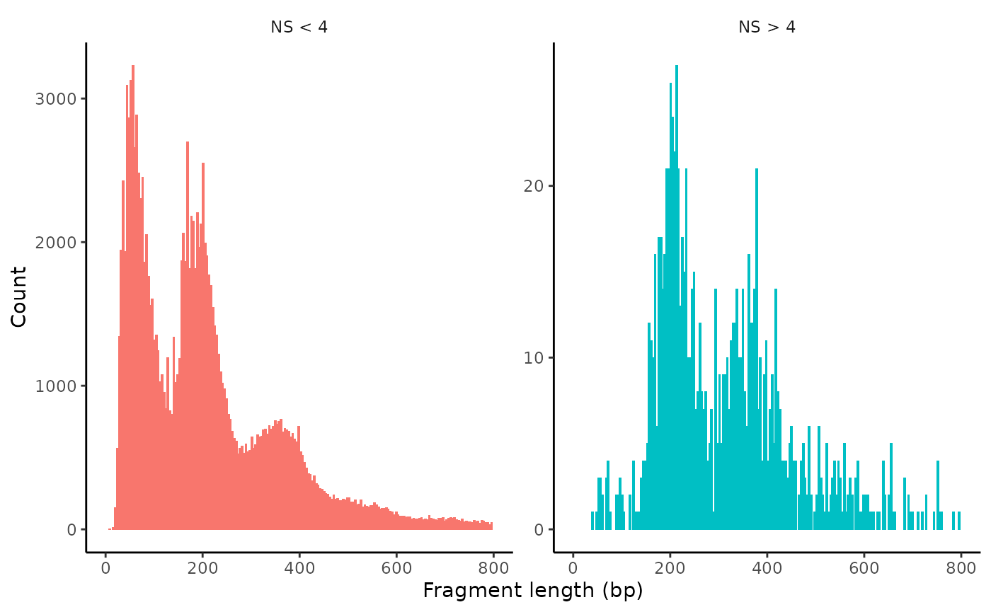
The enrichment of Tn5 integration events at transcriptional start sites (TSSs) can also be an important quality control metric to assess the targeting of Tn5 in ATAC-seq experiments. The ENCODE consortium defined a TSS enrichment score as the number of Tn5 integration site around the TSS normalized to the number of Tn5 integration sites in flanking regions. See the ENCODE documentation for more information about the TSS enrichment score (https://www.encodeproject.org/data-standards/terms/). We can calculate the TSS enrichment score for each cell using the TSSEnrichment() function in Signac.
brain <- TSSEnrichment(brain, fast = FALSE)
brain$high.tss <- ifelse(brain$TSS.enrichment > 2, 'High', 'Low')
TSSPlot(brain, group.by = 'high.tss') + NoLegend()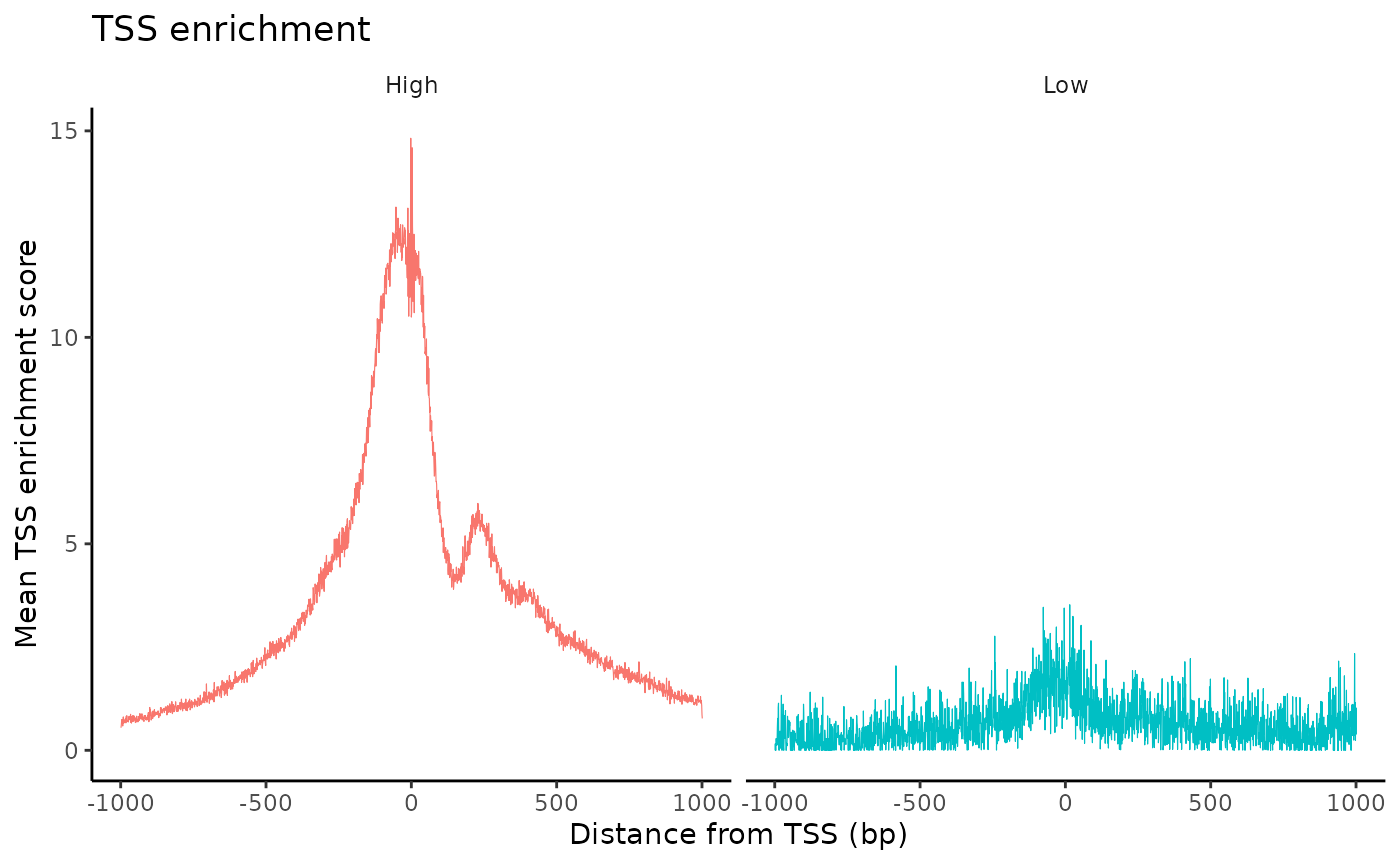
brain$pct_reads_in_peaks <- brain$peak_region_fragments / brain$passed_filters * 100
brain$blacklist_ratio <- brain$blacklist_region_fragments / brain$peak_region_fragments

VlnPlot(
  object = brain,
  features = c('pct_reads_in_peaks', 'peak_region_fragments',
               'TSS.enrichment', 'blacklist_ratio', 'nucleosome_signal'),
  pt.size = 0.1,
  ncol = 5
)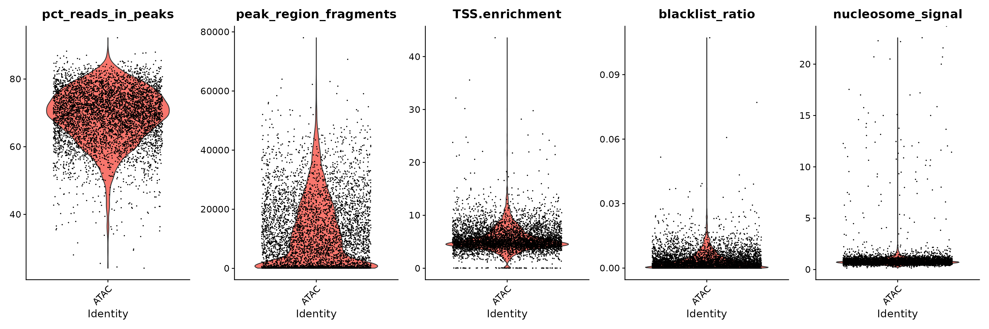
We remove cells that are outliers for these QC metrics.
brain <- subset(
  x = brain,
  subset = peak_region_fragments > 3000 &
    peak_region_fragments < 100000 &
    pct_reads_in_peaks > 40 &
    blacklist_ratio < 0.025 &
    nucleosome_signal < 4 &
    TSS.enrichment > 2
)
brain
## An object of class Seurat
## 157203 features across 3512 samples within 1 assay
## Active assay: peaks (157203 features, 0 variable features)Normalization and linear dimensional reduction
brain <- RunTFIDF(brain)
brain <- FindTopFeatures(brain, min.cutoff = 'q0')
brain <- RunSVD(object = brain)
The first LSI component often captures sequencing depth (technical variation) rather than biological variation. If this is the case, the component should be removed from downstream analysis. We can assess the correlation between each LSI component and sequencing depth using the DepthCor() function:
DepthCor(brain)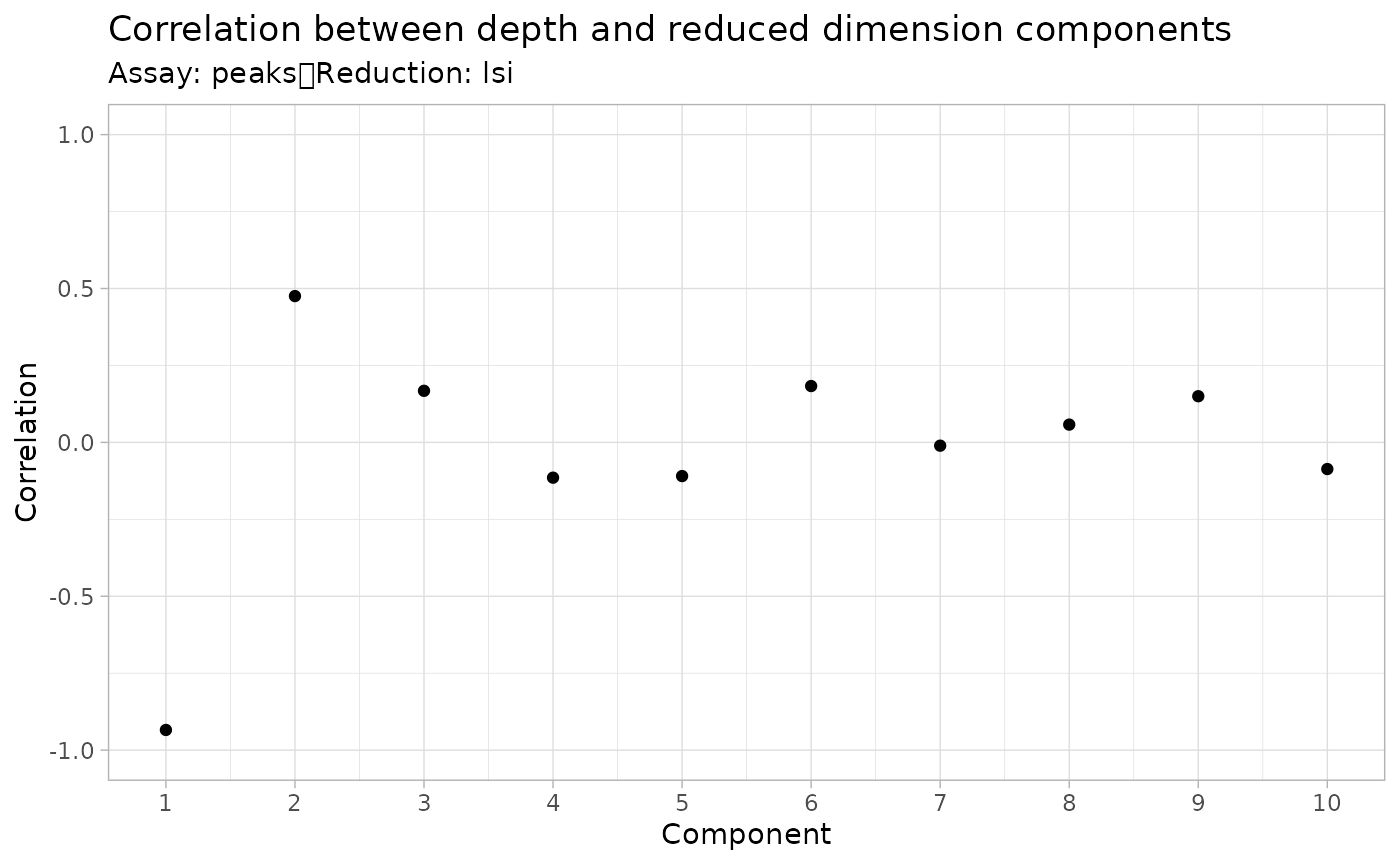
Here we see there is a very strong correlation between the first LSI component and the total number of counts for the cell, so we will perform downstream steps without this component.
Non-linear dimension reduction and clustering
Now that the cells are embedded in a low-dimensional space, we can use methods commonly applied for the analysis of scRNA-seq data to perform graph-based clustering, and non-linear dimension reduction for visualization. The functions RunUMAP(), FindNeighbors(), and FindClusters() all come from the Seurat package.
brain <- RunUMAP(
  object = brain,
  reduction = 'lsi',
  dims = 2:30
)
brain <- FindNeighbors(
  object = brain,
  reduction = 'lsi',
  dims = 2:30
)
brain <- FindClusters(
  object = brain,
  algorithm = 3,
  resolution = 1.2,
  verbose = FALSE
)

DimPlot(object = brain, label = TRUE) + NoLegend()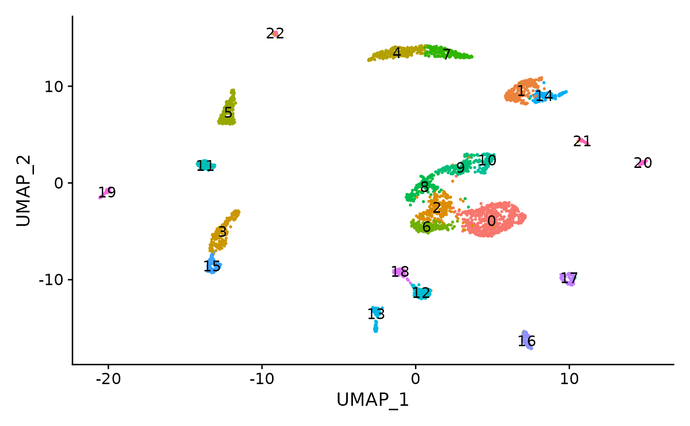
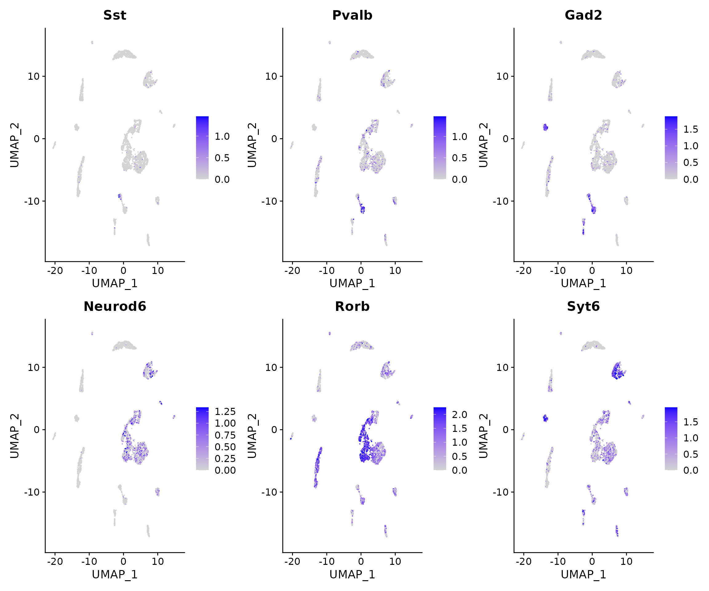
Create a gene activity matrix
# compute gene activities
gene.activities <- GeneActivity(brain)

# add the gene activity matrix to the Seurat object as a new assay
brain[['RNA']] <- CreateAssayObject(counts = gene.activities)
brain <- NormalizeData(
  object = brain,
  assay = 'RNA',
  normalization.method = 'LogNormalize',
  scale.factor = median(brain$nCount_RNA)
)
DefaultAssay(brain) <- 'RNA'
FeaturePlot(
  object = brain,
  features = c('Sst','Pvalb',"Gad2","Neurod6","Rorb","Syt6"),
  pt.size = 0.1,
  max.cutoff = 'q95',
  ncol = 3
)
Integrating with scRNA-seq data
To help interpret the scATAC-seq data, we can classify cells based on an scRNA-seq experiment from the same biological system (the adult mouse brain). We utilize methods for cross-modality integration and label transfer, described here, with a more in-depth tutorial here.
You can download the raw data for this experiment from the Allen Institute website, and view the code used to construct this object on GitHub. Alternatively, you can download the pre-processed Seurat object here.
# Load the pre-processed scRNA-seq data
allen_rna <- readRDS("/home/stuartt/github/chrom/vignette_data/allen_brain.rds")
allen_rna <- FindVariableFeatures(
  object = allen_rna,
  nfeatures = 5000
)

transfer.anchors <- FindTransferAnchors(
  reference = allen_rna,
  query = brain,
  reduction = 'cca',
  dims = 1:40
)

predicted.labels <- TransferData(
  anchorset = transfer.anchors,
  refdata = allen_rna$subclass,
  weight.reduction = brain[['lsi']],
  dims = 2:30
)

brain <- AddMetaData(object = brain, metadata = predicted.labels)
plot1 <- DimPlot(allen_rna, group.by = 'subclass', label = TRUE, repel = TRUE) + NoLegend() + ggtitle('scRNA-seq')
plot2 <- DimPlot(brain, group.by = 'predicted.id', label = TRUE, repel = TRUE) + NoLegend() + ggtitle('scATAC-seq')
plot1 + plot2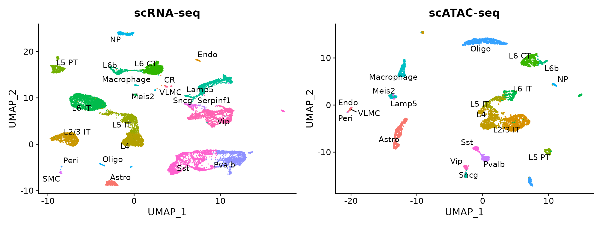
Why did we change default parameters?
We changed default parameters for FindIntegrationAnchors() and FindVariableFeatures() (including more features and dimensions). You can run the analysis both ways, and observe very similar results. However, when using default parameters we mislabel cluster 11 cells as Vip-interneurons, when they are in fact a Meis2 expressing CGE-derived interneuron population recently described by us and others. The reason is that this subset is exceptionally rare in the scRNA-seq data (0.3%), and so the genes define this subset (for example, Meis2) were too lowly expressed to be selected in the initial set of variable features. We therefore need more genes and dimensions to facilitate cross-modality mapping. Interestingly, this subset is 10-fold more abundant in the scATAC-seq data compared to the scRNA-seq data (see this paper for possible explanations.)
You can see that the RNA-based classifications are entirely consistent with the UMAP visualization, computed only on the ATAC-seq data. We can now easily annotate our scATAC-seq derived clusters (alternately, we could use the RNA classifications themselves). We note three small clusters (13, 20, 21) which represent subdivisions of the scRNA-seq labels. Try transferring the cluster label (which shows finer distinctions) from the allen scRNA-seq dataset, to annotate them!
Find differentially accessible peaks between clusters
Here, we find differentially accessible regions between excitatory neurons in different layers of the cortex.
#switch back to working with peaks instead of gene activities
DefaultAssay(brain) <- 'peaks'

da_peaks <- FindMarkers(
  object = brain,
  ident.1 = c("L2/3 IT"),
  ident.2 = c("L4", "L5 IT", "L6 IT"),
  min.pct = 0.4,
  test.use = 'LR',
  latent.vars = 'peak_region_fragments'
)

head(da_peaks)
## p_val avg_log2FC pct.1 pct.2 p_val_adj
## chr4-86523678-86525285 3.413350e-67 0.8098730 0.401 0.036 5.365888e-62
## chr15-87605281-87607659 2.945028e-59 0.7262452 0.485 0.090 4.629672e-54
## chr2-118700082-118704897 5.135950e-57 0.4401448 0.622 0.180 8.073868e-52
## chr3-137056475-137058371 9.571201e-53 0.5114632 0.523 0.103 1.504621e-47
## chr13-69329933-69331707 1.019300e-52 -0.6129178 0.143 0.445 1.602370e-47
## chr10-107751762-107753240 2.126567e-51 0.5680184 0.611 0.185 3.343027e-46
plot1 <- VlnPlot(
  object = brain,
  features = rownames(da_peaks)[1],
  pt.size = 0.1,
  idents = c("L4","L5 IT","L2/3 IT")
)
plot2 <- FeaturePlot(
  object = brain,
  features = rownames(da_peaks)[1],
  pt.size = 0.1,
  max.cutoff = 'q95'
)
plot1 | plot2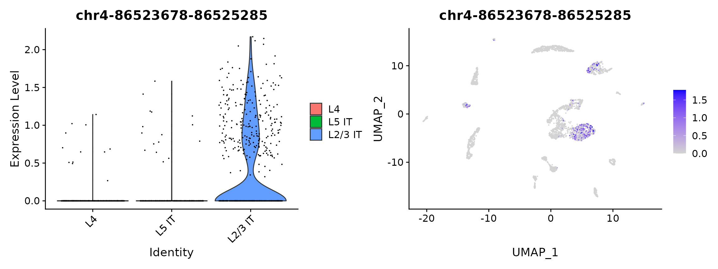
open_l23 <- rownames(da_peaks[da_peaks$avg_log2FC > 0.25, ])
open_l456 <- rownames(da_peaks[da_peaks$avg_log2FC < -0.25, ])
closest_l23 <- ClosestFeature(brain, open_l23)
closest_l456 <- ClosestFeature(brain, open_l456)
head(closest_l23)
## tx_id gene_name gene_id
## ENSMUST00000151481 ENSMUST00000151481 Fam154a ENSMUSG00000028492
## ENSMUSE00000647021 ENSMUST00000068088 Fam19a5 ENSMUSG00000054863
## ENSMUST00000104937 ENSMUST00000104937 Ankrd63 ENSMUSG00000078137
## ENSMUST00000070198 ENSMUST00000070198 Ppp3ca ENSMUSG00000028161
## ENSMUST00000165341 ENSMUST00000165341 Otogl ENSMUSG00000091455
## ENSMUST00000179893 ENSMUST00000179893 Ryr1 ENSMUSG00000030592
## gene_biotype type closest_region
## ENSMUST00000151481 protein_coding gap chr4-86487920-86538964
## ENSMUSE00000647021 protein_coding exon chr15-87625230-87625486
## ENSMUST00000104937 protein_coding cds chr2-118702266-118703438
## ENSMUST00000070198 protein_coding utr chr3-136935226-136937727
## ENSMUST00000165341 protein_coding utr chr10-107762223-107762309
## ENSMUST00000179893 protein_coding cds chr7-29073019-29073139
## query_region distance
## ENSMUST00000151481 chr4-86523678-86525285 0
## ENSMUSE00000647021 chr15-87605281-87607659 17570
## ENSMUST00000104937 chr2-118700082-118704897 0
## ENSMUST00000070198 chr3-137056475-137058371 118747
## ENSMUST00000165341 chr10-107751762-107753240 8982
## ENSMUST00000179893 chr7-29070299-29073172 0
head(closest_l456)## tx_id gene_name gene_id
## ENSMUST00000044081 ENSMUST00000044081 Papd7 ENSMUSG00000034575
## ENSMUST00000084628 ENSMUST00000084628 Hs3st2 ENSMUSG00000046321
## ENSMUST00000022986 ENSMUST00000022986 Fbxo32 ENSMUSG00000022358
## ENSMUST00000114842 ENSMUST00000114842 Anks1 ENSMUSG00000024219
## ENSMUST00000020002 ENSMUST00000020002 Abracl ENSMUSG00000078453
## ENSMUST00000189373 ENSMUST00000189373 Spock1 ENSMUSG00000056222
## gene_biotype type closest_region
## ENSMUST00000044081 protein_coding utr chr13-69497959-69499915
## ENSMUST00000084628 protein_coding cds chr7-121392730-121393214
## ENSMUST00000022986 protein_coding cds chr15-58214496-58214611
## ENSMUST00000114842 protein_coding cds chr17-28007849-28008432
## ENSMUST00000020002 protein_coding utr chr10-18023067-18023252
## ENSMUST00000189373 protein_coding gap chr13-57587734-57696109
## query_region distance
## ENSMUST00000044081 chr13-69329933-69331707 166251
## ENSMUST00000084628 chr7-121391215-121395519 0
## ENSMUST00000022986 chr15-58213714-58216137 0
## ENSMUST00000114842 chr17-28005280-28010176 0
## ENSMUST00000020002 chr10-18020389-18023587 0
## ENSMUST00000189373 chr13-57636759-57639538 0Plotting genomic regions
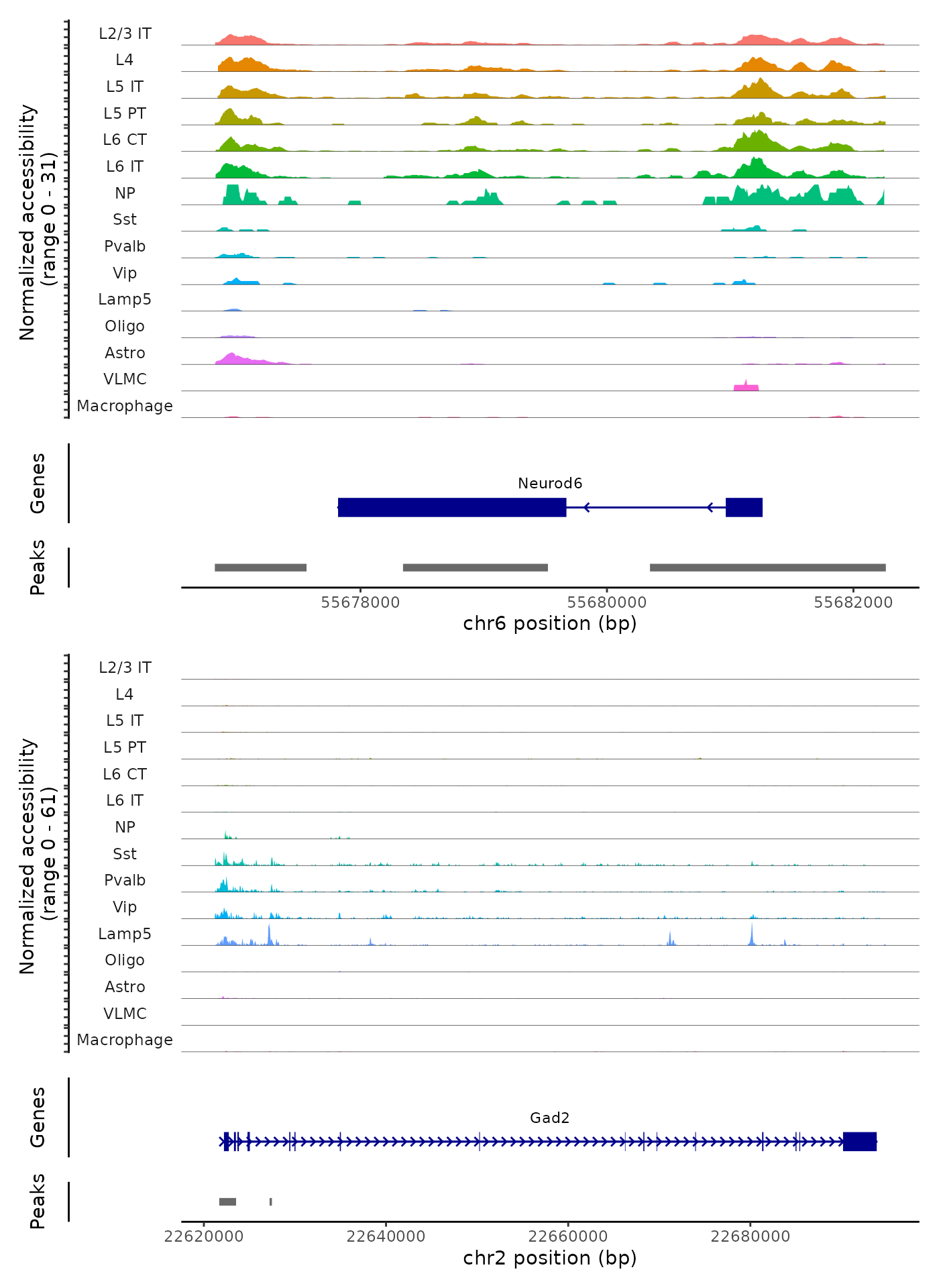
We can also create coverage plots grouped by cluster, cell type, or any other metadata stored in the object for any genomic region using the CoveragePlot() function. These represent pseudo-bulk accessibility tracks, where signal from all cells within a group have been averaged together to visualize the DNA accessibility in a region.
# set plotting order
levels(brain) <- c("L2/3 IT","L4","L5 IT","L5 PT","L6 CT", "L6 IT","NP","Sst","Pvalb","Vip","Lamp5","Meis2","Oligo","Astro","Endo","VLMC","Macrophage")

CoveragePlot(
  object = brain,
  region = c("Neurod6", "Gad2"),
  extend.upstream = 1000,
  extend.downstream = 1000,
  ncol = 1
)
Session Info
## R version 4.0.1 (2020-06-06)
## Platform: x86_64-pc-linux-gnu (64-bit)
## Running under: Ubuntu 18.04.5 LTS
##
## Matrix products: default
## BLAS:   /usr/lib/x86_64-linux-gnu/blas/libblas.so.3.7.1
## LAPACK: /usr/lib/x86_64-linux-gnu/lapack/liblapack.so.3.7.1
##
## locale:
##  [1] LC_CTYPE=en_US.UTF-8       LC_NUMERIC=C
##  [3] LC_TIME=en_US.UTF-8        LC_COLLATE=en_US.UTF-8
##  [5] LC_MONETARY=en_US.UTF-8    LC_MESSAGES=en_US.UTF-8
##  [7] LC_PAPER=en_US.UTF-8       LC_NAME=C
##  [9] LC_ADDRESS=C               LC_TELEPHONE=C
## [11] LC_MEASUREMENT=en_US.UTF-8 LC_IDENTIFICATION=C
##
## attached base packages:
## [1] stats4    parallel  stats     graphics  grDevices utils     datasets
## [8] methods   base
##
## other attached packages:
##  [1] patchwork_1.1.1            ggplot2_3.3.3
##  [3] EnsDb.Mmusculus.v79_2.99.0 ensembldb_2.14.0
##  [5] AnnotationFilter_1.14.0    GenomicFeatures_1.42.3
##  [7] AnnotationDbi_1.52.0       Biobase_2.50.0
##  [9] GenomicRanges_1.42.0       GenomeInfoDb_1.26.5
## [11] IRanges_2.24.1             S4Vectors_0.28.1
## [13] BiocGenerics_0.36.0        SeuratObject_4.0.0
## [15] Seurat_4.0.1.9005          Signac_1.2.0
##
## loaded via a namespace (and not attached):
##   [1] utf8_1.2.1                  reticulate_1.19
##   [3] tidyselect_1.1.0            RSQLite_2.2.7
##   [5] htmlwidgets_1.5.3           grid_4.0.1
##   [7] docopt_0.7.1                BiocParallel_1.24.1
##   [9] Rtsne_0.15                  munsell_0.5.0
##  [11] codetools_0.2-18            ragg_1.1.2
##  [13] ica_1.0-2                   future_1.21.0
##  [15] miniUI_0.1.1.1              withr_2.4.2
##  [17] colorspace_2.0-0            highr_0.9
##  [19] knitr_1.33                  rstudioapi_0.13
##  [21] ROCR_1.0-11                 tensor_1.5
##  [23] listenv_0.8.0               labeling_0.4.2
##  [25] MatrixGenerics_1.2.1        slam_0.1-48
##  [27] GenomeInfoDbData_1.2.4      polyclip_1.10-0
##  [29] bit64_4.0.5                 farver_2.1.0
##  [31] rprojroot_2.0.2             parallelly_1.24.0
##  [33] vctrs_0.3.7                 generics_0.1.0
##  [35] xfun_0.22                   biovizBase_1.38.0
##  [37] BiocFileCache_1.14.0        lsa_0.73.2
##  [39] ggseqlogo_0.1               R6_2.5.0
##  [41] hdf5r_1.3.3                 bitops_1.0-7
##  [43] spatstat.utils_2.1-0        cachem_1.0.4
##  [45] DelayedArray_0.16.3         assertthat_0.2.1
##  [47] promises_1.2.0.1            scales_1.1.1
##  [49] nnet_7.3-15                 gtable_0.3.0
##  [51] globals_0.14.0              goftest_1.2-2
##  [53] rlang_0.4.10                systemfonts_1.0.1
##  [55] RcppRoll_0.3.0              splines_4.0.1
##  [57] rtracklayer_1.50.0          lazyeval_0.2.2
##  [59] dichromat_2.0-0             checkmate_2.0.0
##  [61] spatstat.geom_2.1-0         yaml_2.2.1
##  [63] reshape2_1.4.4              abind_1.4-5
##  [65] backports_1.2.1             httpuv_1.6.0
##  [67] Hmisc_4.5-0                 tools_4.0.1
##  [69] ellipsis_0.3.1              spatstat.core_2.1-2
##  [71] jquerylib_0.1.4             RColorBrewer_1.1-2
##  [73] ggridges_0.5.3              Rcpp_1.0.6
##  [75] plyr_1.8.6                  base64enc_0.1-3
##  [77] progress_1.2.2              zlibbioc_1.36.0
##  [79] purrr_0.3.4                 RCurl_1.98-1.3
##  [81] prettyunits_1.1.1           rpart_4.1-15
##  [83] openssl_1.4.3               deldir_0.2-10
##  [85] pbapply_1.4-3               cowplot_1.1.1
##  [87] zoo_1.8-9                   SummarizedExperiment_1.20.0
##  [89] ggrepel_0.9.1               cluster_2.1.2
##  [91] fs_1.5.0                    magrittr_2.0.1
##  [93] RSpectra_0.16-0             data.table_1.14.0
##  [95] scattermore_0.7             lmtest_0.9-38
##  [97] RANN_2.6.1                  SnowballC_0.7.0
##  [99] ProtGenerics_1.22.0         fitdistrplus_1.1-3
## [101] matrixStats_0.58.0          hms_1.0.0
## [103] mime_0.10                   evaluate_0.14
## [105] xtable_1.8-4                XML_3.99-0.6
## [107] jpeg_0.1-8.1                sparsesvd_0.2
## [109] gridExtra_2.3               compiler_4.0.1
## [111] biomaRt_2.46.3              tibble_3.1.1
## [113] KernSmooth_2.23-18          crayon_1.4.1
## [115] htmltools_0.5.1.1           mgcv_1.8-33
## [117] later_1.2.0                 Formula_1.2-4
## [119] tidyr_1.1.3                 DBI_1.1.1
## [121] tweenr_1.0.2                dbplyr_2.1.1
## [123] MASS_7.3-53.1               rappdirs_0.3.3
## [125] Matrix_1.3-2                igraph_1.2.6
## [127] pkgconfig_2.0.3             pkgdown_1.6.1
## [129] GenomicAlignments_1.26.0    foreign_0.8-81
## [131] plotly_4.9.3                spatstat.sparse_2.0-0
## [133] xml2_1.3.2                  bslib_0.2.4
## [135] XVector_0.30.0              VariantAnnotation_1.36.0
## [137] stringr_1.4.0               digest_0.6.27
## [139] sctransform_0.3.2           RcppAnnoy_0.0.18
## [141] spatstat.data_2.1-0         Biostrings_2.58.0
## [143] rmarkdown_2.7               leiden_0.3.7
## [145] fastmatch_1.1-0             htmlTable_2.1.0
## [147] uwot_0.1.10                 curl_4.3
## [149] shiny_1.6.0                 Rsamtools_2.6.0
## [151] lifecycle_1.0.0             nlme_3.1-152
## [153] jsonlite_1.7.2              BSgenome_1.58.0
## [155] desc_1.3.0                  viridisLite_0.4.0
## [157] askpass_1.1                 fansi_0.4.2
## [159] pillar_1.6.0                lattice_0.20-41
## [161] fastmap_1.1.0               httr_1.4.2
## [163] survival_3.2-11             glue_1.4.2
## [165] qlcMatrix_0.9.7             png_0.1-7
## [167] bit_4.0.4                   ggforce_0.3.3
## [169] stringi_1.5.3               sass_0.3.1
## [171] blob_1.2.1                  textshaping_0.3.3
## [173] latticeExtra_0.6-29         memoise_2.0.0
## [175] dplyr_1.0.5                 irlba_2.3.3
## [177] future.apply_1.7.0