Motif analysis with Signac
Compiled: April 28, 2021
Source:vignettes/motif_vignette.Rmd
motif_vignette.RmdIn this tutorial, we will perform DNA sequence motif analysis in Signac. We will explore two complementary options for performing motif analysis: one by finding overrepresented motifs in a set of differentially accessible peaks, one method performing differential motif activity analysis between groups of cells.
In this demonstration we use data from the adult mouse brain. See our vignette for the code used to generate this object, and links to the raw data. First, load the required packages and the pre-computed Seurat object:
library(Signac)
library(Seurat)
library(JASPAR2020)
library(TFBSTools)
library(BSgenome.Mmusculus.UCSC.mm10)
library(patchwork)
set.seed(1234)
mouse_brain <- readRDS("../vignette_data/adult_mouse_brain.rds")
mouse_brain
## An object of class Seurat
## 179221 features across 3512 samples within 2 assays
## Active assay: peaks (157203 features, 157203 variable features)
## 1 other assay present: RNA
## 2 dimensional reductions calculated: lsi, umap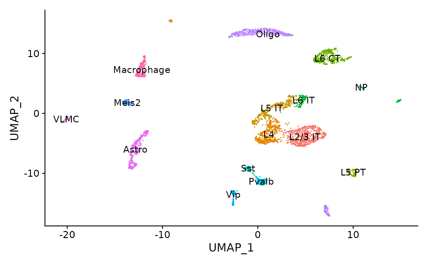
Adding motif information to the Seurat object
To add the DNA sequence motif information required for motif analyses, we can run the AddMotifs() function:
# Get a list of motif position frequency matrices from the JASPAR database
pfm <- getMatrixSet(
  x = JASPAR2020,
  opts = list(species = 9606, all_versions = FALSE)
)

# add motif information
mouse_brain <- AddMotifs(
  object = mouse_brain,
  genome = BSgenome.Mmusculus.UCSC.mm10,
  pfm = pfm
)
To facilitate motif analysis in Signac, we have create the Motif class to store all the required information, including a list of position weight matrices (PWMs) or position frequency matrices (PFMs) and a motif occurrence matrix. Here, the AddMotifs() function construct a Motif object and adds it to our mouse brain dataset, along with other information such as the base composition of each peak. A motif object can be added to any Seurat assay using the SetAssayData() function. See the object interaction vignette for more information.
Finding overrepresented motifs
To identify potentially important cell-type-specific regulatory sequences, we can search for DNA motifs that are overrepresented in a set of peaks that are differentially accessible between cell types.
Here, we find differentially accessible peaks between Pvalb and Sst inhibitory interneurons. We then perform a hypergeometric test to test the probability of observing the motif at the given frequency by chance, comparing with a background set of peaks matched for GC content.
da_peaks <- FindMarkers(
  object = mouse_brain,
  ident.1 = 'Pvalb',
  ident.2 = 'Sst',
  only.pos = TRUE,
  test.use = 'LR',
  latent.vars = 'nCount_peaks'
)

# get top differentially accessible peaks
top.da.peak <- rownames(da_peaks[da_peaks$p_val < 0.005, ])
Optional: choosing a set of background peaks
Matching the set of background peaks is essential when finding enriched DNA sequence motifs. By default, we choose a set of peaks matched for GC content, but it can be sometimes be beneficial to further restrict the background peaks to those that are accessible in the groups of cells compared when finding differentially accessible peaks.
The AccessiblePeaks() function can be used to find a set of peaks that are open in a subset of cells. We can use this function to first restrict the set of possible background peaks to those peaks that were open in the set of cells compared in FindMarkers(), and then create a GC-content-matched set of peaks from this larger set using MatchRegionStats().
# find peaks open in Pvalb or Sst cells
open.peaks <- AccessiblePeaks(mouse_brain, idents = c("Pvalb", "Sst"))

# match the overall GC content in the peak set
meta.feature <- GetAssayData(mouse_brain, assay = "peaks", slot = "meta.features")
peaks.matched <- MatchRegionStats(
  meta.feature = meta.feature[open.peaks, ],
  query.feature = meta.feature[top.da.peak, ],
  n = 50000
)
## Matching GC.percent distributionpeaks.matched can then be used as the background peak set by setting background=peaks.matched in FindMotifs().
# test enrichment
enriched.motifs <- FindMotifs(
  object = mouse_brain,
  features = top.da.peak
)
## Selecting background regions to match input sequence characteristics## Matching GC.percent distribution## Testing motif enrichment in 2436 regions| motif | observed | background | percent.observed | percent.background | fold.enrichment | pvalue | motif.name | |
|---|---|---|---|---|---|---|---|---|
| MA0497.1 | MA0497.1 | 1038 | 9027 | 42.61084 | 22.5675 | 1.888151 | 0 | MEF2C |
| MA0052.4 | MA0052.4 | 978 | 8738 | 40.14778 | 21.8450 | 1.837848 | 0 | MEF2A |
| MA0773.1 | MA0773.1 | 707 | 5382 | 29.02299 | 13.4550 | 2.157041 | 0 | MEF2D |
| MA1151.1 | MA1151.1 | 510 | 3237 | 20.93596 | 8.0925 | 2.587082 | 0 | RORC |
| MA1150.1 | MA1150.1 | 493 | 3068 | 20.23810 | 7.6700 | 2.638604 | 0 | RORB |
| MA0660.1 | MA0660.1 | 599 | 4383 | 24.58949 | 10.9575 | 2.244079 | 0 | MEF2B |
We can also plot the position weight matrices for the motifs, so we can visualize the different motif sequences.
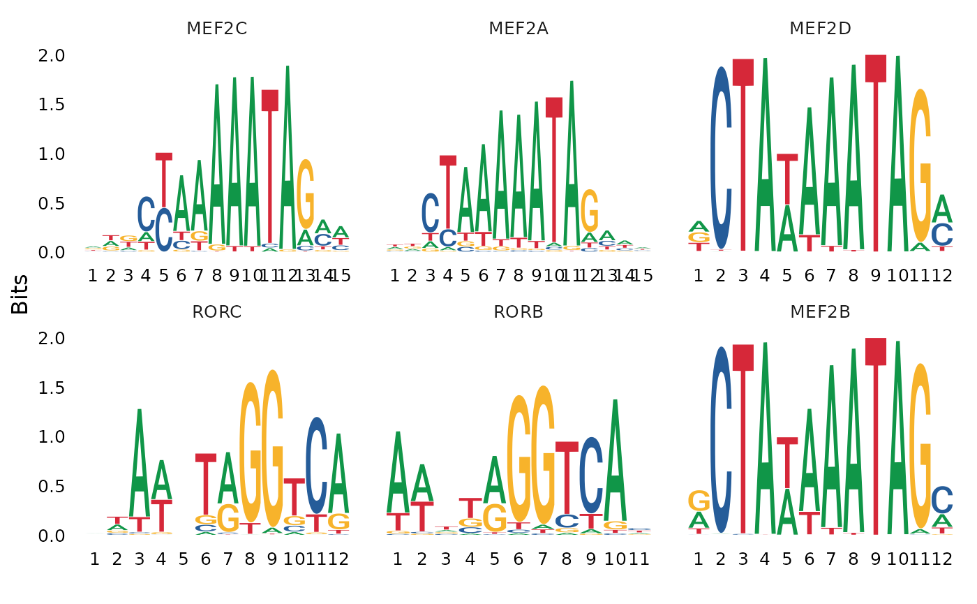
We and others have previously shown that Mef-family motifs, particularly Mef2c, are enriched in Pvalb-specific peaks in scATAC-seq data (https://doi.org/10.1016/j.cell.2019.05.031; https://doi.org/10.1101/615179), and further shown that Mef2c is required for the development of Pvalb interneurons (https://www.nature.com/articles/nature25999). Here our results are consistent with these findings, and we observe a strong enrichment of Mef-family motifs in the top results from FindMotifs().
Computing motif activities
We can also compute a per-cell motif activity score by running chromVAR. This allows us to visualize motif activities per cell, and also provides an alternative method of identifying differentially-active motifs between cell types.
ChromVAR identifies motifs associated with variability in chromatin accessibility between cells. See the chromVAR paper for a complete description of the method.
mouse_brain <- RunChromVAR(
  object = mouse_brain,
  genome = BSgenome.Mmusculus.UCSC.mm10
)

DefaultAssay(mouse_brain) <- 'chromvar'

# look at the activity of Mef2c
p2 <- FeaturePlot(
  object = mouse_brain,
  features = "MA0497.1",
  min.cutoff = 'q10',
  max.cutoff = 'q90',
  pt.size = 0.1
)
p1 + p2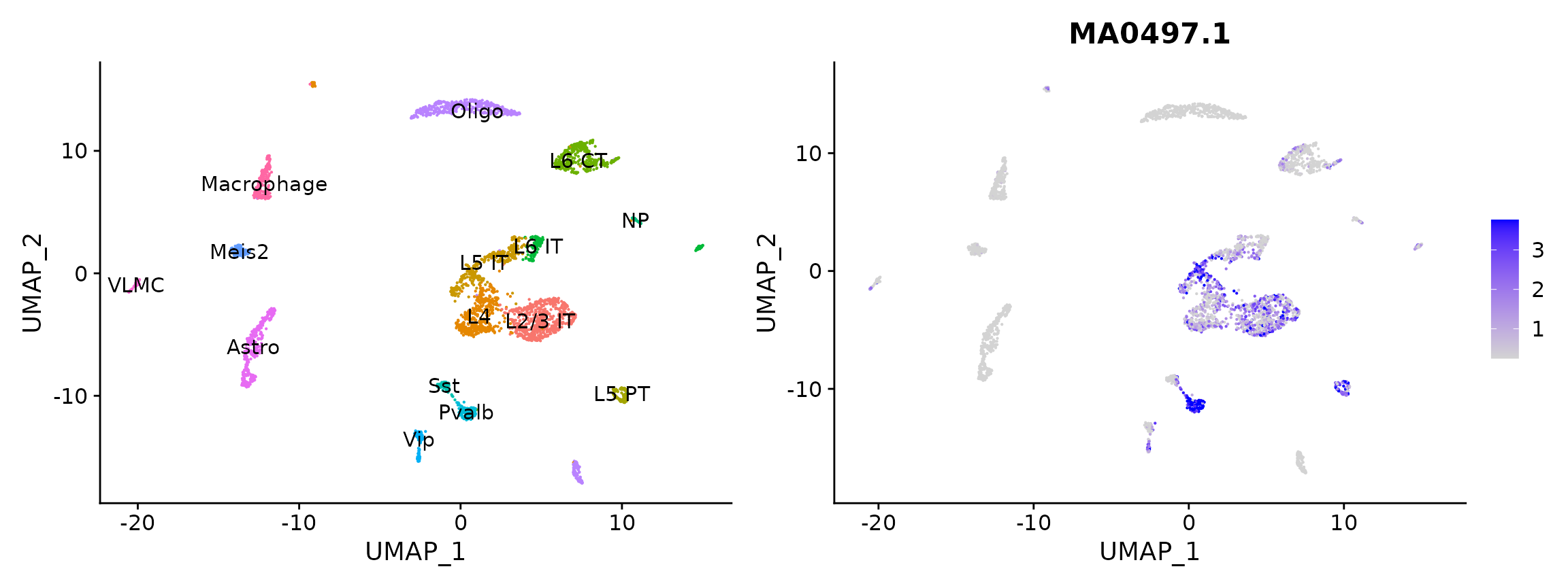
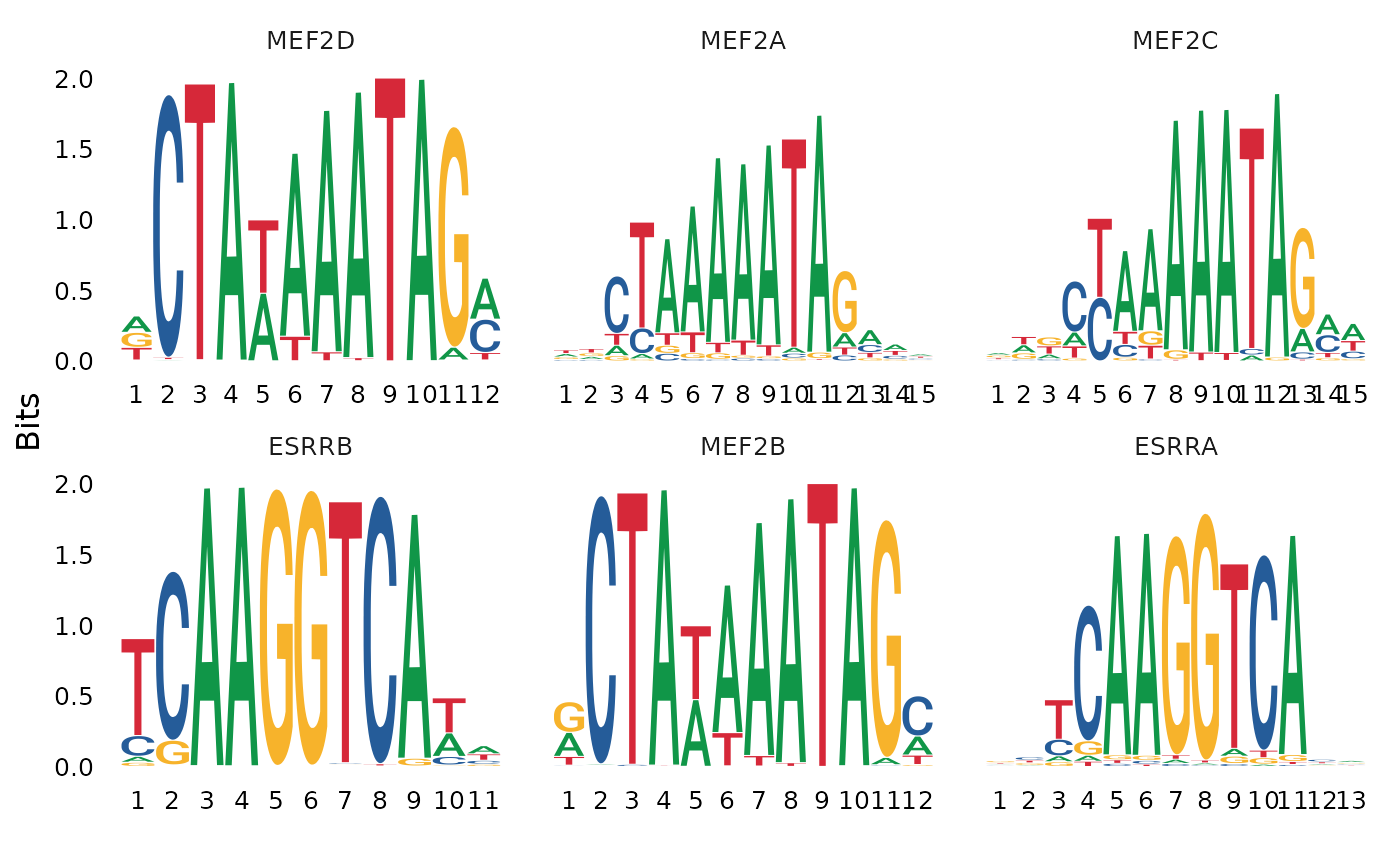
We can also directly test for differential activity scores between cell types. This tends to give similar results as performing an enrichment test on differentially accessible peaks between the cell types (shown above).
differential.activity <- FindMarkers(
  object = mouse_brain,
  ident.1 = 'Pvalb',
  ident.2 = 'Sst',
  only.pos = TRUE,
  test.use = 'LR',
  latent.vars = 'nCount_peaks'
)

MotifPlot(
  object = mouse_brain,
  motifs = head(rownames(differential.activity)),
  assay = 'peaks'
)
Session Info
## R version 4.0.1 (2020-06-06)
## Platform: x86_64-pc-linux-gnu (64-bit)
## Running under: Ubuntu 18.04.5 LTS
##
## Matrix products: default
## BLAS:   /usr/lib/x86_64-linux-gnu/blas/libblas.so.3.7.1
## LAPACK: /usr/lib/x86_64-linux-gnu/lapack/liblapack.so.3.7.1
##
## locale:
##  [1] LC_CTYPE=en_US.UTF-8       LC_NUMERIC=C
##  [3] LC_TIME=en_US.UTF-8        LC_COLLATE=en_US.UTF-8
##  [5] LC_MONETARY=en_US.UTF-8    LC_MESSAGES=en_US.UTF-8
##  [7] LC_PAPER=en_US.UTF-8       LC_NAME=C
##  [9] LC_ADDRESS=C               LC_TELEPHONE=C
## [11] LC_MEASUREMENT=en_US.UTF-8 LC_IDENTIFICATION=C
##
## attached base packages:
## [1] stats4    parallel  stats     graphics  grDevices utils     datasets
## [8] methods   base
##
## other attached packages:
##  [1] patchwork_1.1.1                    BSgenome.Mmusculus.UCSC.mm10_1.4.0
##  [3] BSgenome_1.58.0                    rtracklayer_1.50.0
##  [5] Biostrings_2.58.0                  XVector_0.30.0
##  [7] GenomicRanges_1.42.0               GenomeInfoDb_1.26.5
##  [9] IRanges_2.24.1                     S4Vectors_0.28.1
## [11] BiocGenerics_0.36.0                TFBSTools_1.28.0
## [13] JASPAR2020_0.99.10                 SeuratObject_4.0.0
## [15] Seurat_4.0.1.9005                  Signac_1.2.0
##
## loaded via a namespace (and not attached):
##   [1] utf8_1.2.1                  R.utils_2.10.1
##   [3] reticulate_1.19             tidyselect_1.1.0
##   [5] AnnotationDbi_1.52.0        poweRlaw_0.70.6
##   [7] RSQLite_2.2.7               htmlwidgets_1.5.3
##   [9] grid_4.0.1                  docopt_0.7.1
##  [11] BiocParallel_1.24.1         Rtsne_0.15
##  [13] munsell_0.5.0               codetools_0.2-18
##  [15] ragg_1.1.2                  ica_1.0-2
##  [17] DT_0.18                     future_1.21.0
##  [19] miniUI_0.1.1.1              colorspace_2.0-0
##  [21] chromVAR_1.12.0             Biobase_2.50.0
##  [23] highr_0.9                   knitr_1.33
##  [25] ROCR_1.0-11                 tensor_1.5
##  [27] listenv_0.8.0               labeling_0.4.2
##  [29] MatrixGenerics_1.2.1        slam_0.1-48
##  [31] GenomeInfoDbData_1.2.4      polyclip_1.10-0
##  [33] bit64_4.0.5                 farver_2.1.0
##  [35] rprojroot_2.0.2             parallelly_1.24.0
##  [37] vctrs_0.3.7                 generics_0.1.0
##  [39] xfun_0.22                   lsa_0.73.2
##  [41] ggseqlogo_0.1               R6_2.5.0
##  [43] bitops_1.0-7                spatstat.utils_2.1-0
##  [45] cachem_1.0.4                DelayedArray_0.16.3
##  [47] assertthat_0.2.1            promises_1.2.0.1
##  [49] scales_1.1.1                gtable_0.3.0
##  [51] globals_0.14.0              goftest_1.2-2
##  [53] seqLogo_1.56.0              rlang_0.4.10
##  [55] systemfonts_1.0.1           RcppRoll_0.3.0
##  [57] splines_4.0.1               lazyeval_0.2.2
##  [59] spatstat.geom_2.1-0         yaml_2.2.1
##  [61] reshape2_1.4.4              abind_1.4-5
##  [63] httpuv_1.6.0                tools_4.0.1
##  [65] nabor_0.5.0                 ggplot2_3.3.3
##  [67] ellipsis_0.3.1              spatstat.core_2.1-2
##  [69] jquerylib_0.1.4             RColorBrewer_1.1-2
##  [71] ggridges_0.5.3              Rcpp_1.0.6
##  [73] plyr_1.8.6                  zlibbioc_1.36.0
##  [75] purrr_0.3.4                 RCurl_1.98-1.3
##  [77] rpart_4.1-15                deldir_0.2-10
##  [79] pbapply_1.4-3               cowplot_1.1.1
##  [81] zoo_1.8-9                   SummarizedExperiment_1.20.0
##  [83] ggrepel_0.9.1               cluster_2.1.2
##  [85] fs_1.5.0                    motifmatchr_1.12.0
##  [87] magrittr_2.0.1              data.table_1.14.0
##  [89] scattermore_0.7             lmtest_0.9-38
##  [91] RANN_2.6.1                  SnowballC_0.7.0
##  [93] fitdistrplus_1.1-3          matrixStats_0.58.0
##  [95] hms_1.0.0                   mime_0.10
##  [97] evaluate_0.14               xtable_1.8-4
##  [99] XML_3.99-0.6                sparsesvd_0.2
## [101] gridExtra_2.3               compiler_4.0.1
## [103] tibble_3.1.1                KernSmooth_2.23-18
## [105] crayon_1.4.1                R.oo_1.24.0
## [107] htmltools_0.5.1.1           mgcv_1.8-33
## [109] later_1.2.0                 tidyr_1.1.3
## [111] DBI_1.1.1                   tweenr_1.0.2
## [113] MASS_7.3-53.1               Matrix_1.3-2
## [115] readr_1.4.0                 R.methodsS3_1.8.1
## [117] igraph_1.2.6                pkgconfig_2.0.3
## [119] pkgdown_1.6.1               GenomicAlignments_1.26.0
## [121] TFMPvalue_0.0.8             plotly_4.9.3
## [123] spatstat.sparse_2.0-0       annotate_1.68.0
## [125] bslib_0.2.4                 DirichletMultinomial_1.32.0
## [127] stringr_1.4.0               digest_0.6.27
## [129] sctransform_0.3.2           RcppAnnoy_0.0.18
## [131] pracma_2.3.3                CNEr_1.26.0
## [133] spatstat.data_2.1-0         rmarkdown_2.7
## [135] leiden_0.3.7                fastmatch_1.1-0
## [137] uwot_0.1.10                 shiny_1.6.0
## [139] Rsamtools_2.6.0             gtools_3.8.2
## [141] lifecycle_1.0.0             nlme_3.1-152
## [143] jsonlite_1.7.2              desc_1.3.0
## [145] viridisLite_0.4.0           fansi_0.4.2
## [147] pillar_1.6.0                lattice_0.20-41
## [149] KEGGREST_1.30.1             GO.db_3.12.1
## [151] fastmap_1.1.0               httr_1.4.2
## [153] survival_3.2-11             glue_1.4.2
## [155] qlcMatrix_0.9.7             png_0.1-7
## [157] bit_4.0.4                   ggforce_0.3.3
## [159] stringi_1.5.3               sass_0.3.1
## [161] blob_1.2.1                  textshaping_0.3.3
## [163] caTools_1.18.2              memoise_2.0.0
## [165] dplyr_1.0.5                 irlba_2.3.3
## [167] future.apply_1.7.0