Joint RNA and ATAC analysis: 10x multiomic
Compiled: April 28, 2021
Source:vignettes/pbmc_multiomic.Rmd
pbmc_multiomic.RmdIn this vignette, we’ll demonstrate how to jointly analyze a single-cell dataset measuring both DNA accessibility and gene expression in the same cells using Signac and Seurat.
To demonstrate we’ll use a dataset provided by 10x Genomics for human PBMCs. You can download the required data here:
library(Signac)
library(Seurat)
library(EnsDb.Hsapiens.v86)
library(BSgenome.Hsapiens.UCSC.hg38)

set.seed(1234)
# load the RNA and ATAC data
counts <- Read10X_h5("../vignette_data/multiomic/pbmc_granulocyte_sorted_10k_filtered_feature_bc_matrix.h5")
fragpath <- "../vignette_data/multiomic/pbmc_granulocyte_sorted_10k_atac_fragments.tsv.gz"
# get gene annotations for hg38
annotation <- GetGRangesFromEnsDb(ensdb = EnsDb.Hsapiens.v86)
seqlevelsStyle(annotation) <- "UCSC"
genome(annotation) <- "hg38"

# create a Seurat object containing the RNA adata
pbmc <- CreateSeuratObject(
  counts = counts$`Gene Expression`,
  assay = "RNA"
)

# create ATAC assay and add it to the object
pbmc[["ATAC"]] <- CreateChromatinAssay(
  counts = counts$Peaks,
  sep = c(":", "-"),
  fragments = fragpath,
  annotation = annotation
)
pbmc## An object of class Seurat
## 144978 features across 11909 samples within 2 assays
## Active assay: RNA (36601 features, 0 variable features)
## 1 other assay present: ATACQuality control
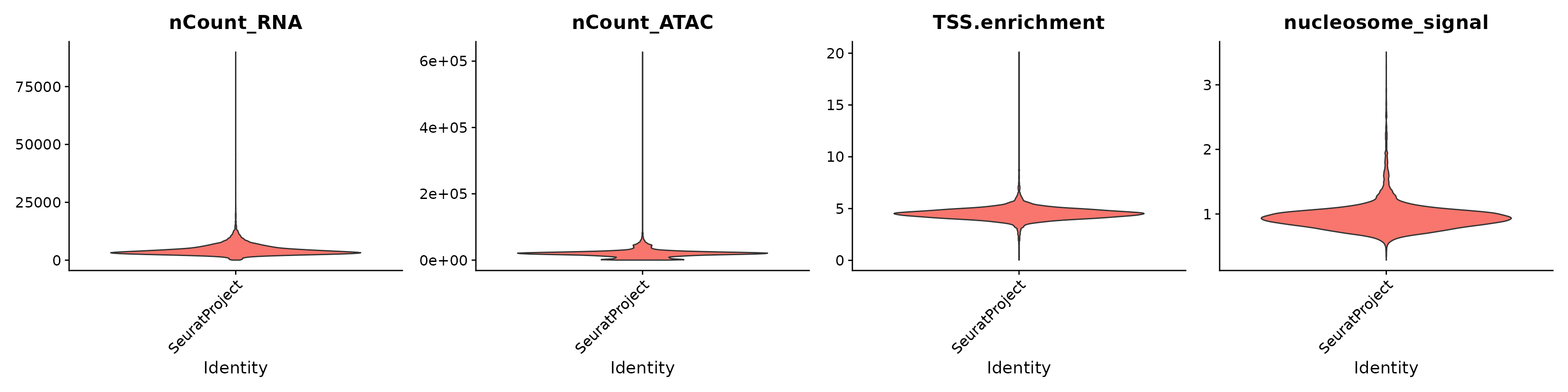
We can compute per-cell quality control metrics using the DNA accessibility data and remove cells that are outliers for these metrics, as well as cells with low or unusually high counts for either the RNA or ATAC assay.
DefaultAssay(pbmc) <- "ATAC"

pbmc <- NucleosomeSignal(pbmc)
pbmc <- TSSEnrichment(pbmc)

VlnPlot(
  object = pbmc,
  features = c("nCount_RNA", "nCount_ATAC", "TSS.enrichment", "nucleosome_signal"),
  ncol = 4,
  pt.size = 0
)
# filter out low quality cells
pbmc <- subset(
  x = pbmc,
  subset = nCount_ATAC < 100000 &
    nCount_RNA < 25000 &
    nCount_ATAC > 1000 &
    nCount_RNA > 1000 &
    nucleosome_signal < 2 &
    TSS.enrichment > 1
)
pbmc
## An object of class Seurat
## 144978 features across 11331 samples within 2 assays
## Active assay: ATAC (108377 features, 0 variable features)
## 1 other assay present: RNAPeak calling
The set of peaks identified using Cellranger often merges distinct peaks that are close together. This can create a problem for certain analyses, particularly motif enrichment analysis and peak-to-gene linkage. To identify a more accurate set of peaks, we can call peaks using MACS2 with the CallPeaks() function. Here we call peaks on all cells together, but we could identify peaks for each group of cells separately by setting the group.by parameter, and this can help identify peaks specific to rare cell populations.
# call peaks using MACS2
peaks <- CallPeaks(pbmc, macs2.path = "/home/stuartt/miniconda3/envs/signac/bin/macs2")

# remove peaks on nonstandard chromosomes and in genomic blacklist regions
peaks <- keepStandardChromosomes(peaks, pruning.mode = "coarse")
peaks <- subsetByOverlaps(x = peaks, ranges = blacklist_hg38_unified, invert = TRUE)

# quantify counts in each peak
macs2_counts <- FeatureMatrix(
  fragments = Fragments(pbmc),
  features = peaks,
  cells = colnames(pbmc)
)

# create a new assay using the MACS2 peak set and add it to the Seurat object
pbmc[["peaks"]] <- CreateChromatinAssay(
  counts = macs2_counts,
  fragments = fragpath,
  annotation = annotation
)
Gene expression data processing
We can normalize the gene expression data using SCTransform, and reduce the dimensionality using PCA.
DefaultAssay(pbmc) <- "RNA"
pbmc <- SCTransform(pbmc)
pbmc <- RunPCA(pbmc)
DNA accessibility data processing
Here we process the DNA accessibility assay the same way we would process a scATAC-seq dataset, by performing latent semantic indexing (LSI).
DefaultAssay(pbmc) <- "peaks"
pbmc <- FindTopFeatures(pbmc, min.cutoff = 5)
pbmc <- RunTFIDF(pbmc)
pbmc <- RunSVD(pbmc)
Annotating cell types
To annotate cell types in the dataset we can transfer cell labels from an existing PBMC reference dataset using tools in the Seurat package. See the Seurat reference mapping vignette for more information.
We’ll use an annotated PBMC reference dataset from Hao et al. (2020), available for download here: https://atlas.fredhutch.org/data/nygc/multimodal/pbmc_multimodal.h5seurat
Note that the SeuratDisk package is required to load the reference dataset. Installation instructions for SeuratDisk can be found here.
library(SeuratDisk)

# load PBMC reference
reference <- LoadH5Seurat("../vignette_data/multiomic/pbmc_multimodal.h5seurat")

DefaultAssay(pbmc) <- "SCT"

# transfer cell type labels from reference to query
transfer_anchors <- FindTransferAnchors(
  reference = reference,
  query = pbmc,
  normalization.method = "SCT",
  reference.reduction = "spca",
  recompute.residuals = FALSE,
  dims = 1:50
)

predictions <- TransferData(
  anchorset = transfer_anchors,
  refdata = reference$celltype.l2,
  weight.reduction = pbmc[['pca']],
  dims = 1:50
)

pbmc <- AddMetaData(
  object = pbmc,
  metadata = predictions
)

# set the cell identities to the cell type predictions
Idents(pbmc) <- "predicted.id"

# set a reasonable order for cell types to be displayed when plotting
levels(pbmc) <- c("CD4 Naive", "CD4 TCM", "CD4 CTL", "CD4 TEM", "CD4 Proliferating",
                  "CD8 Naive", "dnT",
                 "CD8 TEM", "CD8 TCM", "CD8 Proliferating", "MAIT", "NK", "NK_CD56bright",
                 "NK Proliferating", "gdT",
                 "Treg", "B naive", "B intermediate", "B memory", "Plasmablast",
                 "CD14 Mono", "CD16 Mono",
                 "cDC1", "cDC2", "pDC", "HSPC", "Eryth", "ASDC", "ILC", "Platelet")
Joint UMAP visualization
Using the weighted nearest neighbor methods in Seurat v4, we can compute a joint neighbor graph that represent both the gene expression and DNA accessibility measurements.
# build a joint neighbor graph using both assays
pbmc <- FindMultiModalNeighbors(
  object = pbmc,
  reduction.list = list("pca", "lsi"),
  dims.list = list(1:50, 2:40),
  modality.weight.name = "RNA.weight",
  verbose = TRUE
)

# build a joint UMAP visualization
pbmc <- RunUMAP(
  object = pbmc,
  nn.name = "weighted.nn",
  assay = "RNA",
  verbose = TRUE
)

DimPlot(pbmc, label = TRUE, repel = TRUE, reduction = "umap") + NoLegend()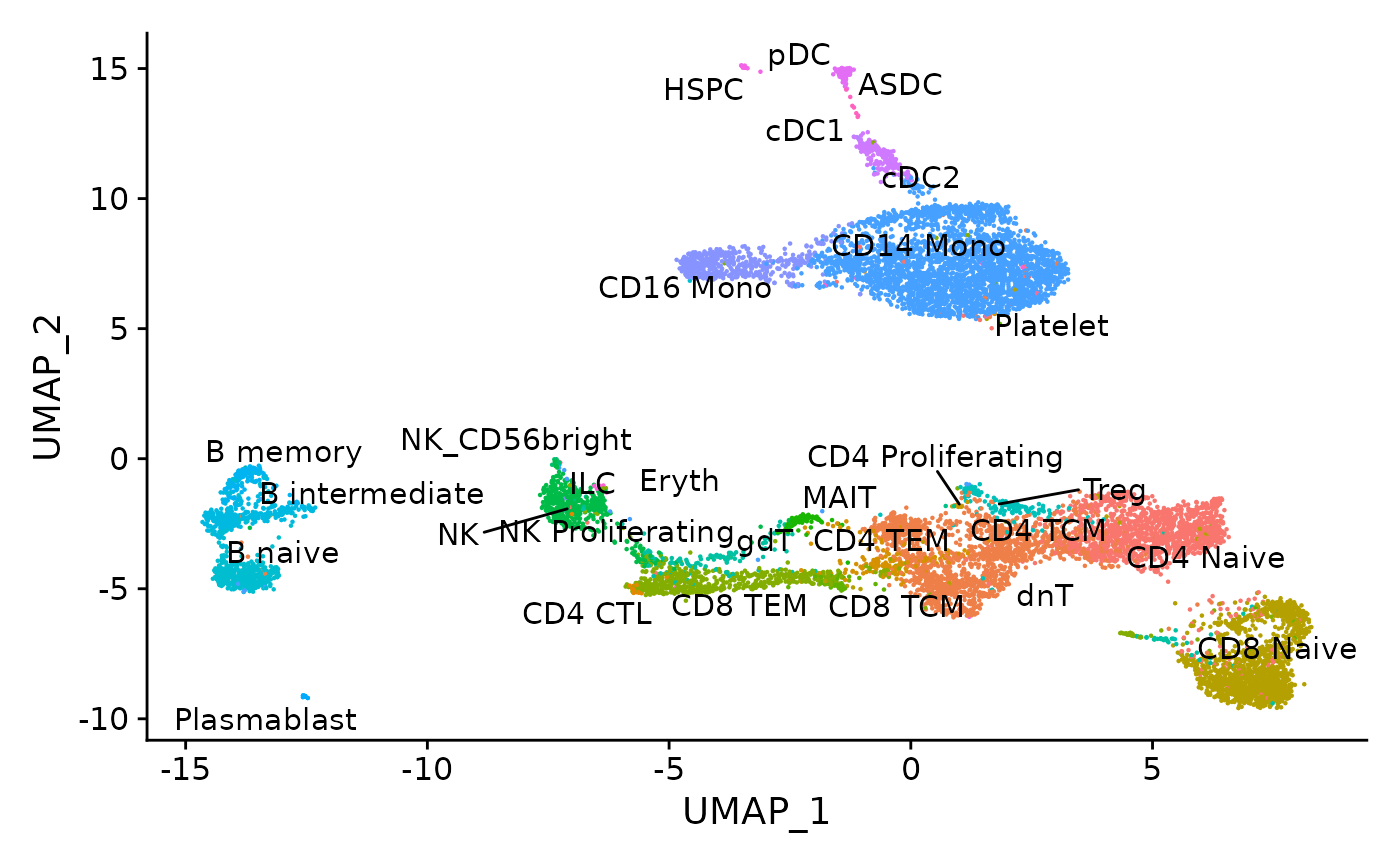
Linking peaks to genes
For each gene, we can find the set of peaks that may regulate the gene by by computing the correlation between gene expression and accessibility at nearby peaks, and correcting for bias due to GC content, overall accessibility, and peak size. See the Signac paper for a full description of the method we use to link peaks to genes.
Running this step on the whole genome can be time consuming, so here we demonstrate peak-gene links for a subset of genes as an example. The same function can be used to find links for all genes by omitting the genes.use parameter:
DefaultAssay(pbmc) <- "peaks"

# first compute the GC content for each peak
pbmc <- RegionStats(pbmc, genome = BSgenome.Hsapiens.UCSC.hg38)

# link peaks to genes
pbmc <- LinkPeaks(
  object = pbmc,
  peak.assay = "peaks",
  expression.assay = "SCT",
  genes.use = c("LYZ", "MS4A1")
)
We can visualize these links using the CoveragePlot() function, or alternatively we could use the CoverageBrowser() function in an interactive analysis:
idents.plot <- c("B naive", "B intermediate", "B memory",
                 "CD14 Mono", "CD16 Mono", "CD8 TEM", "CD8 Naive")

p1 <- CoveragePlot(
  object = pbmc,
  region = "MS4A1",
  features = "MS4A1",
  expression.assay = "SCT",
  idents = idents.plot,
  extend.upstream = 500,
  extend.downstream = 10000
)

p2 <- CoveragePlot(
  object = pbmc,
  region = "LYZ",
  features = "LYZ",
  expression.assay = "SCT",
  idents = idents.plot,
  extend.upstream = 8000,
  extend.downstream = 5000
)

patchwork::wrap_plots(p1, p2, ncol = 1)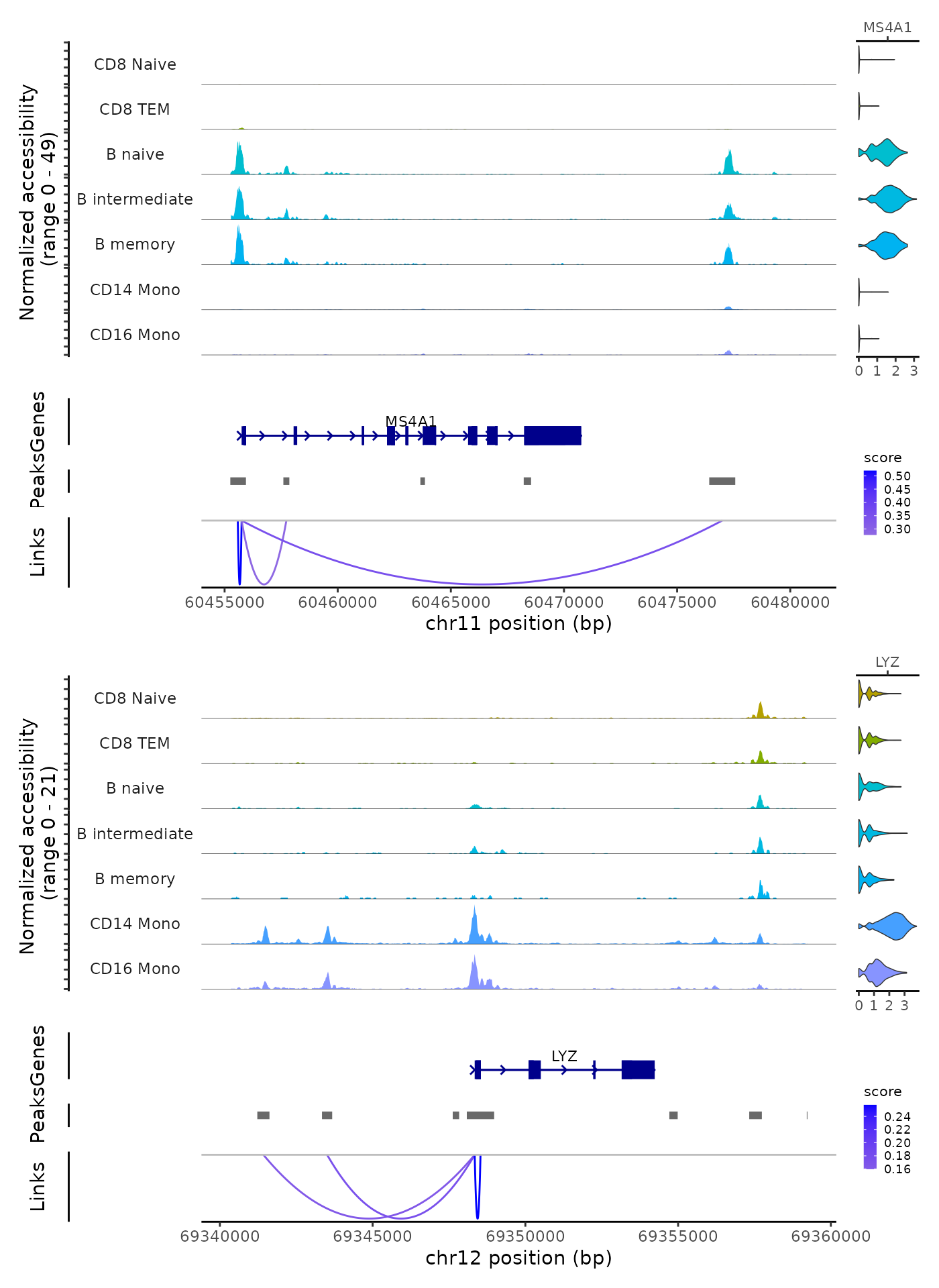
Session Info
## R version 4.0.1 (2020-06-06)
## Platform: x86_64-pc-linux-gnu (64-bit)
## Running under: Ubuntu 18.04.5 LTS
##
## Matrix products: default
## BLAS:   /usr/lib/x86_64-linux-gnu/blas/libblas.so.3.7.1
## LAPACK: /usr/lib/x86_64-linux-gnu/lapack/liblapack.so.3.7.1
##
## locale:
##  [1] LC_CTYPE=en_US.UTF-8       LC_NUMERIC=C
##  [3] LC_TIME=en_US.UTF-8        LC_COLLATE=en_US.UTF-8
##  [5] LC_MONETARY=en_US.UTF-8    LC_MESSAGES=en_US.UTF-8
##  [7] LC_PAPER=en_US.UTF-8       LC_NAME=C
##  [9] LC_ADDRESS=C               LC_TELEPHONE=C
## [11] LC_MEASUREMENT=en_US.UTF-8 LC_IDENTIFICATION=C
##
## attached base packages:
## [1] stats4    parallel  stats     graphics  grDevices utils     datasets
## [8] methods   base
##
## other attached packages:
##  [1] SeuratDisk_0.0.0.9016             BSgenome.Hsapiens.UCSC.hg38_1.4.3
##  [3] BSgenome_1.58.0                   rtracklayer_1.50.0
##  [5] Biostrings_2.58.0                 XVector_0.30.0
##  [7] EnsDb.Hsapiens.v86_2.99.0         ensembldb_2.14.0
##  [9] AnnotationFilter_1.14.0           GenomicFeatures_1.42.3
## [11] AnnotationDbi_1.52.0              Biobase_2.50.0
## [13] GenomicRanges_1.42.0              GenomeInfoDb_1.26.5
## [15] IRanges_2.24.1                    S4Vectors_0.28.1
## [17] BiocGenerics_0.36.0               SeuratObject_4.0.0
## [19] Seurat_4.0.1.9005                 Signac_1.2.0
##
## loaded via a namespace (and not attached):
##   [1] utf8_1.2.1                  reticulate_1.19
##   [3] tidyselect_1.1.0            RSQLite_2.2.7
##   [5] htmlwidgets_1.5.3           grid_4.0.1
##   [7] docopt_0.7.1                BiocParallel_1.24.1
##   [9] Rtsne_0.15                  munsell_0.5.0
##  [11] codetools_0.2-18            ragg_1.1.2
##  [13] ica_1.0-2                   future_1.21.0
##  [15] miniUI_0.1.1.1              withr_2.4.2
##  [17] colorspace_2.0-0            highr_0.9
##  [19] knitr_1.33                  rstudioapi_0.13
##  [21] ROCR_1.0-11                 tensor_1.5
##  [23] listenv_0.8.0               labeling_0.4.2
##  [25] MatrixGenerics_1.2.1        slam_0.1-48
##  [27] GenomeInfoDbData_1.2.4      polyclip_1.10-0
##  [29] bit64_4.0.5                 farver_2.1.0
##  [31] rprojroot_2.0.2             parallelly_1.24.0
##  [33] vctrs_0.3.7                 generics_0.1.0
##  [35] xfun_0.22                   biovizBase_1.38.0
##  [37] BiocFileCache_1.14.0        lsa_0.73.2
##  [39] ggseqlogo_0.1               R6_2.5.0
##  [41] hdf5r_1.3.3                 bitops_1.0-7
##  [43] spatstat.utils_2.1-0        cachem_1.0.4
##  [45] DelayedArray_0.16.3         assertthat_0.2.1
##  [47] promises_1.2.0.1            scales_1.1.1
##  [49] nnet_7.3-15                 gtable_0.3.0
##  [51] globals_0.14.0              goftest_1.2-2
##  [53] rlang_0.4.10                systemfonts_1.0.1
##  [55] RcppRoll_0.3.0              splines_4.0.1
##  [57] lazyeval_0.2.2              dichromat_2.0-0
##  [59] checkmate_2.0.0             spatstat.geom_2.1-0
##  [61] yaml_2.2.1                  reshape2_1.4.4
##  [63] abind_1.4-5                 backports_1.2.1
##  [65] httpuv_1.6.0                Hmisc_4.5-0
##  [67] tools_4.0.1                 ggplot2_3.3.3
##  [69] ellipsis_0.3.1              spatstat.core_2.1-2
##  [71] jquerylib_0.1.4             RColorBrewer_1.1-2
##  [73] ggridges_0.5.3              Rcpp_1.0.6
##  [75] plyr_1.8.6                  base64enc_0.1-3
##  [77] progress_1.2.2              zlibbioc_1.36.0
##  [79] purrr_0.3.4                 RCurl_1.98-1.3
##  [81] prettyunits_1.1.1           rpart_4.1-15
##  [83] openssl_1.4.3               deldir_0.2-10
##  [85] pbapply_1.4-3               cowplot_1.1.1
##  [87] zoo_1.8-9                   SummarizedExperiment_1.20.0
##  [89] ggrepel_0.9.1               cluster_2.1.2
##  [91] fs_1.5.0                    magrittr_2.0.1
##  [93] RSpectra_0.16-0             data.table_1.14.0
##  [95] scattermore_0.7             lmtest_0.9-38
##  [97] RANN_2.6.1                  SnowballC_0.7.0
##  [99] ProtGenerics_1.22.0         fitdistrplus_1.1-3
## [101] matrixStats_0.58.0          hms_1.0.0
## [103] patchwork_1.1.1             mime_0.10
## [105] evaluate_0.14               xtable_1.8-4
## [107] XML_3.99-0.6                jpeg_0.1-8.1
## [109] sparsesvd_0.2               gridExtra_2.3
## [111] compiler_4.0.1              biomaRt_2.46.3
## [113] tibble_3.1.1                KernSmooth_2.23-18
## [115] crayon_1.4.1                htmltools_0.5.1.1
## [117] mgcv_1.8-33                 later_1.2.0
## [119] Formula_1.2-4               tidyr_1.1.3
## [121] DBI_1.1.1                   tweenr_1.0.2
## [123] dbplyr_2.1.1                MASS_7.3-53.1
## [125] rappdirs_0.3.3              Matrix_1.3-2
## [127] cli_2.5.0                   igraph_1.2.6
## [129] pkgconfig_2.0.3             pkgdown_1.6.1
## [131] GenomicAlignments_1.26.0    foreign_0.8-81
## [133] plotly_4.9.3                spatstat.sparse_2.0-0
## [135] xml2_1.3.2                  bslib_0.2.4
## [137] VariantAnnotation_1.36.0    stringr_1.4.0
## [139] digest_0.6.27               sctransform_0.3.2
## [141] RcppAnnoy_0.0.18            spatstat.data_2.1-0
## [143] rmarkdown_2.7               leiden_0.3.7
## [145] fastmatch_1.1-0             htmlTable_2.1.0
## [147] uwot_0.1.10                 curl_4.3
## [149] shiny_1.6.0                 Rsamtools_2.6.0
## [151] lifecycle_1.0.0             nlme_3.1-152
## [153] jsonlite_1.7.2              desc_1.3.0
## [155] viridisLite_0.4.0           askpass_1.1
## [157] fansi_0.4.2                 pillar_1.6.0
## [159] lattice_0.20-41             fastmap_1.1.0
## [161] httr_1.4.2                  survival_3.2-11
## [163] glue_1.4.2                  qlcMatrix_0.9.7
## [165] png_0.1-7                   bit_4.0.4
## [167] ggforce_0.3.3               stringi_1.5.3
## [169] sass_0.3.1                  blob_1.2.1
## [171] textshaping_0.3.3           latticeExtra_0.6-29
## [173] memoise_2.0.0               dplyr_1.0.5
## [175] irlba_2.3.3                 future.apply_1.7.0