Analyzing PBMC scATAC-seq
Compiled: July 06, 2020
Source:vignettes/pbmc_vignette.Rmd
pbmc_vignette.RmdFor this tutorial, we will be analyzing a single-cell ATAC-seq dataset of human peripheral blood mononuclear cells (PBMCs) provided by 10x Genomics. The following files are used in this vignette, all available through the 10x Genomics website:
- The Raw data
- The Metadata
- The fragments file
- The fragments file index
First load in Signac, Seurat, and some other packages we will be using for analyzing human data.
library(Signac)
library(Seurat)
library(GenomeInfoDb)
library(EnsDb.Hsapiens.v75)
library(ggplot2)
library(patchwork)
set.seed(1234)
Quickstart
The vignette below presents a detailed workflow for the pre-processing, QC, clustering, visualization, integration, and interpretation of single-cell ATAC-seq data. While there are many steps (some of which are computationally intensive), we note that the core analytical components are similar to single-cell RNA-seq, and can be run quickly in a few lines. For example, the following lines encapsulate our scATAC-seq workflow (but does not include the calculation of advanced QC metrics, or integration with scRNA-seq data).
library(dplyr)

counts <- Read10X_h5(filename = "/home/stuartt/github/chrom/vignette_data/atac_v1_pbmc_10k_filtered_peak_bc_matrix.h5")
metadata <- read.csv(
  file = "/home/stuartt/github/chrom/vignette_data/atac_v1_pbmc_10k_singlecell.csv",
  header = TRUE,
  row.names = 1
)

pbmc_fast <- CreateSeuratObject(counts = counts,meta.data = metadata) %>%
  subset(peak_region_fragments > 1000) %>%
  RunTFIDF() %>%
  FindTopFeatures(cutoff = 'q75') %>%
  RunSVD(reduction.name='lsi') %>%
  FindNeighbors(reduction='lsi', dims=2:30) %>%
  FindClusters(resolution = 0.5,verbose = FALSE) %>%
  RunUMAP(reduction='lsi', dims=2:30)

DimPlot(pbmc_fast, label = FALSE)
Below, we describe these steps in detail, beginning with pre-processing.
Pre-processing workflow
When pre-processing chromatin data, Signac uses information from two related input files, both of which are created by CellRanger:
Peak/Cell matrix. This is analogous to the gene expression count matrix used to analyze single-cell RNA-seq. However, instead of genes, each row of the matrix represents a region of the genome (a ‘peak’), that is predicted to represent a region of open chromatin. Each value in the matrix represents the number of Tn5 cut sites for each single barcode (i.e. cell) that map within each peak. You can find more detail on the 10X Website.
Fragment file. This represents a full list of all unique fragments across all single cells. It is a substantially larger file, is slower to work with, and is stored on-disk (instead of in memory). However, the advantage of retaining this file is that it contains all fragments associated with each single cell, as opposed to only reads that map to peaks.
For most analyses we work with the peak/cell matrix, but for some (e.g. creating a ‘Gene Activity Matrix’), we find that restricting only to reads in peaks can adversely affect results. We therefore use both files in this vignette. We start by creating a Seurat object using the peak/cell matrix, and store the path to the fragment file on disk in the Seurat object:
counts <- Read10X_h5(filename = "/home/stuartt/github/chrom/vignette_data/atac_v1_pbmc_10k_filtered_peak_bc_matrix.h5")
metadata <- read.csv(
  file = "/home/stuartt/github/chrom/vignette_data/atac_v1_pbmc_10k_singlecell.csv",
  header = TRUE,
  row.names = 1
)

pbmc <- CreateSeuratObject(
  counts = counts,
  assay = 'peaks',
  project = 'ATAC',
  min.cells = 1,
  meta.data = metadata
)
## Warning in CreateSeuratObject.default(counts = counts, assay = "peaks", : Some
## cells in meta.data not present in provided counts matrix
fragment.path <- '/home/stuartt/github/chrom/vignette_data/atac_v1_pbmc_10k_fragments.tsv.gz' pbmc <- SetFragments( object = pbmc, file = fragment.path )
pbmc## An object of class Seurat
## 89307 features across 8728 samples within 1 assay
## Active assay: peaks (89307 features, 0 variable features)Optional step: Filtering the fragment file
To make downstream steps that use this file faster, we can filter the fragments file to contain only reads from cells that we retain in the analysis. This is optional, but slow, and only needs to be performed once. Running this command writes a new file to disk and indexes the file so it is ready to be used by Signac.
fragment_file_filtered <- "/home/stuartt/github/chrom/vignette_data/atac_v1_pbmc_10k_filtered_fragments.tsv"
FilterFragments(
  fragment.path = fragment.path,
  cells = colnames(pbmc),
  output.path = fragment_file_filtered
)
pbmc <- SetFragments(object = pbmc, file = paste0(fragment_file_filtered, '.bgz'))
Computing QC Metrics
We can now compute some QC metrics for the scATAC-seq experiment. We currently suggest the following metrics below to assess data quality. As with scRNA-seq, the expected range of values for these parameters will vary depending on your biological system, cell viability, etc.
Nucleosome banding pattern: The histogram of fragment sizes (determined from the paired-end sequencing reads) should exhibit a strong nucleosome banding pattern. We calculate this per single cell, and quantify the approximate ratio of mononucleosomal to nucleosome-free fragments (stored as
nucleosome_signal). Note that by default, this is calculated only on chr1 reads (see theregionparameter) to save time.Transcriptional start site (TSS) enrichment score. The ENCODE project has defined an ATAC-seq targeting score based on the ratio of fragments centered at the TSS to fragments in TSS-flanking regions (see https://www.encodeproject.org/data-standards/terms/). Poor ATAC-seq experiments typically will have a low TSS enrichment score. We can compute this metric for each cell with the
TSSEnrichmentfunction, and the results are stored in metadata under the column nameTSS.enrichment.Total number of fragments in peaks: A measure of cellular sequencing depth / complexity. Cells with very few reads may need to be excluded due to low sequencing depth. Cells with extremely high levels may represent doublets or nuclear clumps.
Fraction of fragments in peaks. Represents the fraction of total fragments that fall within ATAC-seq peaks. Cells with low values (i.e. <15-20%) often represent low-quality cells or technical artifacts that should be removed.
Ratio reads in ‘blacklist’ sites. The ENCODE project has provided a list of blacklist regions, representing reads which are often associated with artifactual signal. Cells with a high proportion of reads mapping to these areas (compared to reads mapping to peaks) often represent technical artifacts and should be removed. ENCODE blacklist regions for human (hg19 and GRCh38), mouse (mm10), Drosophila (dm3), and C. elegans (ce10) are included in the Signac package.
Note that the last three metrics can be obtained from the output of CellRanger (which is stored in the object metadata), but can also be calculated for non-10x datasets using Signac (more information at the end of this document).
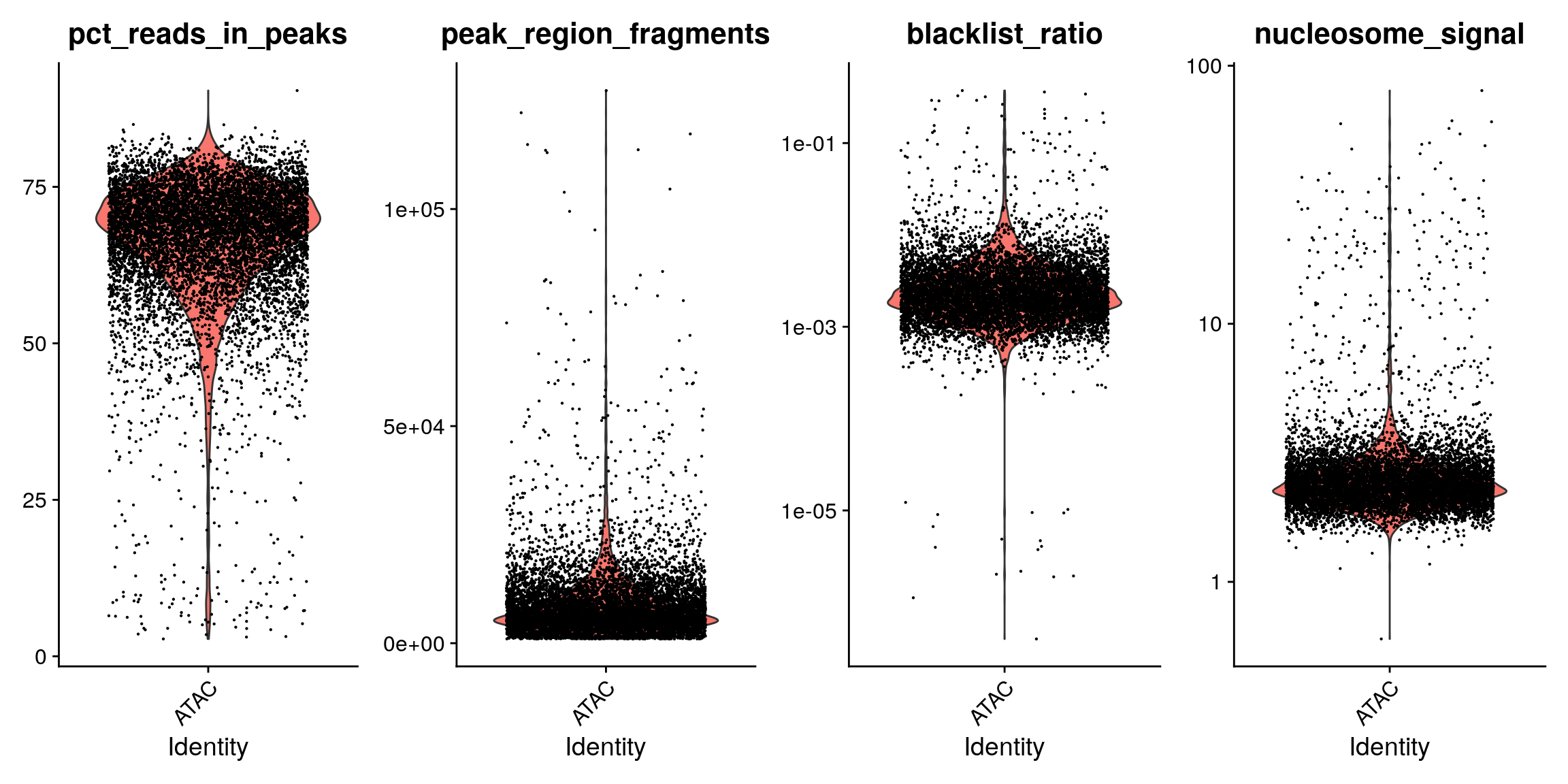
pbmc <- NucleosomeSignal(object = pbmc)
pbmc$pct_reads_in_peaks <- pbmc$peak_region_fragments / pbmc$passed_filters * 100
pbmc$blacklist_ratio <- pbmc$blacklist_region_fragments / pbmc$peak_region_fragments

p1 <- VlnPlot(pbmc, c('pct_reads_in_peaks', 'peak_region_fragments'), pt.size = 0.1)
p2 <- VlnPlot(pbmc, c('blacklist_ratio', 'nucleosome_signal'), pt.size = 0.1) & scale_y_log10()

p1 | p2
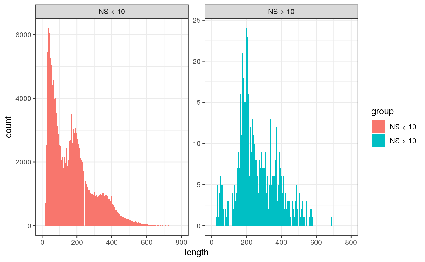
We can also look at the fragment length periodicity for all the cells, and group by cells with high or low nucleosomal signal strength. You can see that cells which are outliers for the mononucleosomal/ nucleosome-free ratio (based off the plots above) have different banding patterns. The remaining cells exhibit a pattern that is typical for a successful ATAC-seq experiment.
pbmc$nucleosome_group <- ifelse(pbmc$nucleosome_signal > 10, 'NS > 10', 'NS < 10')
FragmentHistogram(object = pbmc, group.by = 'nucleosome_group')
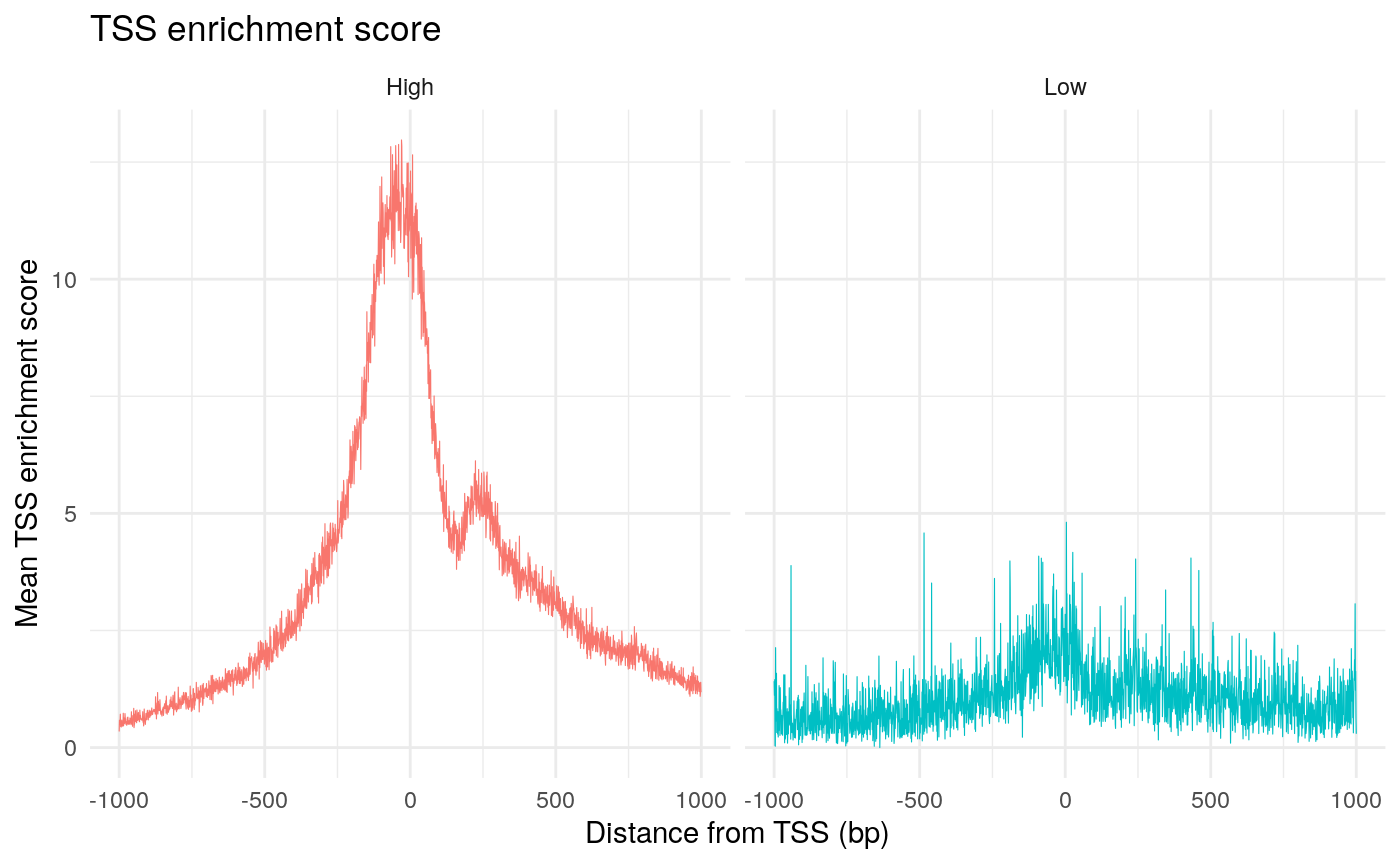
The enrichment of Tn5 integration events at transcriptional start sites (TSSs) can also be an important quality control metric to assess the targeting of Tn5 in ATAC-seq experiments. The ENCODE consortium defined a TSS enrichment score as the number of Tn5 integration site around the TSS normalized to the number of Tn5 integration sites in flanking regions. See the ENCODE documentation for more information about the TSS enrichment score (https://www.encodeproject.org/data-standards/terms/). We can calculate the TSS enrichment score for each cell using the TSSEnrichment function in Signac.
# create granges object with TSS positions
gene.ranges <- genes(EnsDb.Hsapiens.v75)
seqlevelsStyle(gene.ranges) <- 'UCSC'
gene.ranges <- gene.ranges[gene.ranges$gene_biotype == 'protein_coding', ]
gene.ranges <- keepStandardChromosomes(gene.ranges, pruning.mode = 'coarse')

tss.ranges <- resize(gene.ranges, width = 1, fix = "start")
seqlevelsStyle(tss.ranges) <- 'UCSC'
tss.ranges <- keepStandardChromosomes(tss.ranges, pruning.mode = 'coarse')

# to save time use the first 2000 TSSs
pbmc <- TSSEnrichment(object = pbmc, tss.positions = tss.ranges[1:2000])
pbmc$high.tss <- ifelse(pbmc$TSS.enrichment > 2, 'High', 'Low')
TSSPlot(pbmc, group.by = 'high.tss') + ggtitle("TSS enrichment score") + NoLegend()
Finally we remove cells that are outliers for these QC metrics.
pbmc <- subset(
  x = pbmc,
  subset = peak_region_fragments > 3000 &
    peak_region_fragments < 20000 &
    pct_reads_in_peaks > 15 &
    blacklist_ratio < 0.05 &
    nucleosome_signal < 10 &
    TSS.enrichment > 2
)
pbmc
## An object of class Seurat
## 89307 features across 7057 samples within 1 assay
## Active assay: peaks (89307 features, 0 variable features)
Normalization and linear dimensional reduction
Normalization: Signac performs term frequency-inverse document frequency (TF-IDF) normalization. This is a two-step normalization procedure, that both normalizes across cells to correct for differences in cellular sequencing depth, and across peaks to give higher values to more rare peaks.
Feature selection: The largely binary nature of scATAC-seq data makes it challenging to perform ‘variable’ feature selection, as we do for scRNA-seq. Instead, we can choose to use only the top n% of features (peaks) for dimensional reduction, or remove features present in less that n cells with the
FindTopFeaturesfunction. Here, we will all features, though we note that we see very similar results when using only a subset of features (try setting min.cutoff to ‘q75’ to use the top 25% all peaks), with faster runtimes. Features used for dimensional reduction are automatically set asVariableFeaturesfor the Seurat object by this function.Dimensional reduction: We next run a singular value decomposition (SVD) on the TD-IDF normalized matrix, using the features (peaks) selected above. This returns a low-dimensional representation of the object (for users who are more familiar with scRNA-seq, you can think of this as analogous to the output of PCA).
pbmc <- RunTFIDF(pbmc)
pbmc <- FindTopFeatures(pbmc, min.cutoff = 'q0')
pbmc <- RunSVD(
  object = pbmc,
  assay = 'peaks',
  reduction.key = 'LSI_',
  reduction.name = 'lsi'
)
The first LSI component often captures sequencing depth (technical variation) rather than biological variation. If this is the case, the component should be removed from downstream analysis. We can assess the correlation between each LSI component and sequencing depth using the DepthCor function:
DepthCor(pbmc)
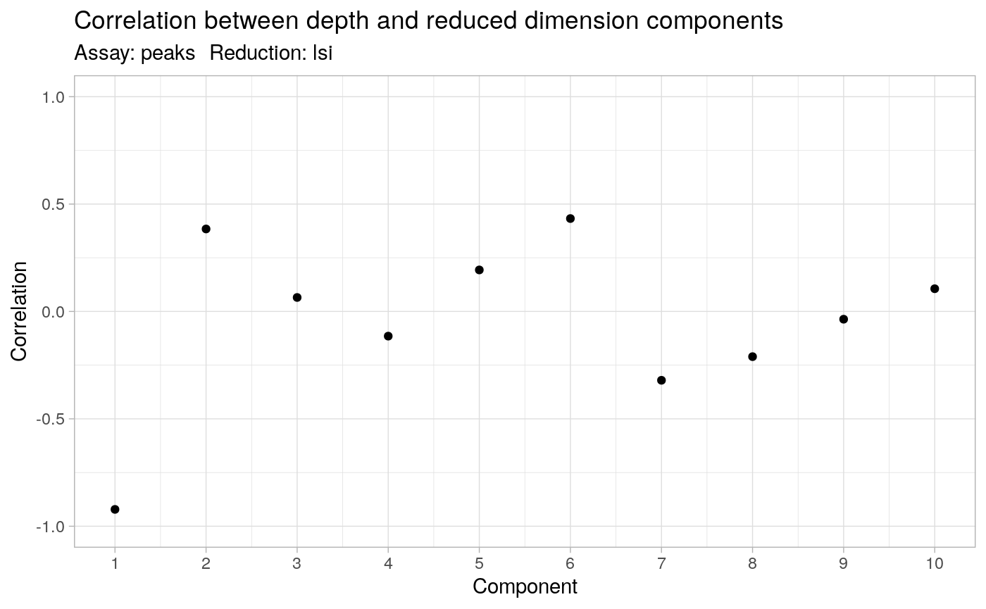
Here we see there is a very strong correlation between the first LSI component and the total number of counts for the cell, so we will perform downstream steps without this component.
Non-linear dimension reduction and clustering
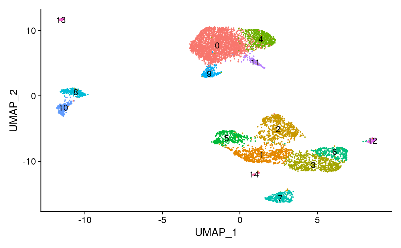
Now that the cells are embedded in a low-dimensional space, we can use methods commonly applied for the analysis of scRNA-seq data to perform graph-based clustering, and non-linear dimension reduction for visualization. The functions RunUMAP, FindNeighbors, and FindClusters all come from the Seurat package.
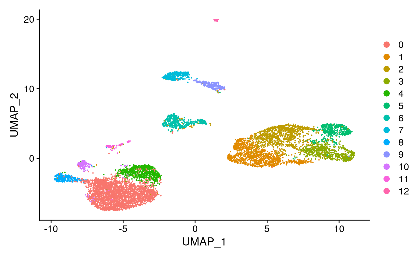
pbmc <- RunUMAP(object = pbmc, reduction = 'lsi', dims = 2:30)
pbmc <- FindNeighbors(object = pbmc, reduction = 'lsi', dims = 2:30)
pbmc <- FindClusters(object = pbmc, verbose = FALSE, algorithm = 3)
DimPlot(object = pbmc, label = TRUE) + NoLegend()
Create a gene activity matrix
The UMAP visualization reveals the presence of multiple cell groups in human blood. If you are familiar with our scRNA-seq analyses of PBMC, you may even recognize the presence of certain myeloid and lymphoid populations in the scATAC-seq data. However, annotating and interpreting clusters is more challenging in scATAC-seq data, as much less is known about the functional roles of noncoding genomic regions than is known about protein coding regions (genes).
However, we can try to quantify the activity of each gene in the genome by assessing the chromatin accessibility associated with each gene, and create a new gene activity assay derived from the scATAC-seq data. Here we will use a simple approach of summing the reads intersecting the gene body and promoter region (we also recommend exploring the Cicero tool, which can accomplish a similar goal).
To create a gene activity matrix, we extract gene coordinates for the human genome from EnsembleDB, and extend them to include the 2kb upstream region (as promoter accessibility is often correlated with gene expression). We then count the number of fragments for each cell that map to each of these regions, using the using the FeatureMatrix function. This takes any set of genomic coordinates, counts the number of reads intersecting these coordinates in each cell, and returns a sparse matrix.
# Extend coordinates upstream to include the promoter
genebodyandpromoter.coords <- Extend(x = gene.ranges, upstream = 2000, downstream = 0)

# create a gene by cell matrix
gene.activities <- FeatureMatrix(
  fragments = fragment.path,
  features = genebodyandpromoter.coords,
  cells = colnames(pbmc),
  chunk = 20
)

# convert rownames from chromsomal coordinates into gene names
gene.key <- genebodyandpromoter.coords$gene_name
names(gene.key) <- GRangesToString(grange = genebodyandpromoter.coords)
rownames(gene.activities) <- gene.key[rownames(gene.activities)]
# add the gene activity matrix to the Seurat object as a new assay, and normalize it
pbmc[['RNA']] <- CreateAssayObject(counts = gene.activities)
pbmc <- NormalizeData(
  object = pbmc,
  assay = 'RNA',
  normalization.method = 'LogNormalize',
  scale.factor = median(pbmc$nCount_RNA)
)
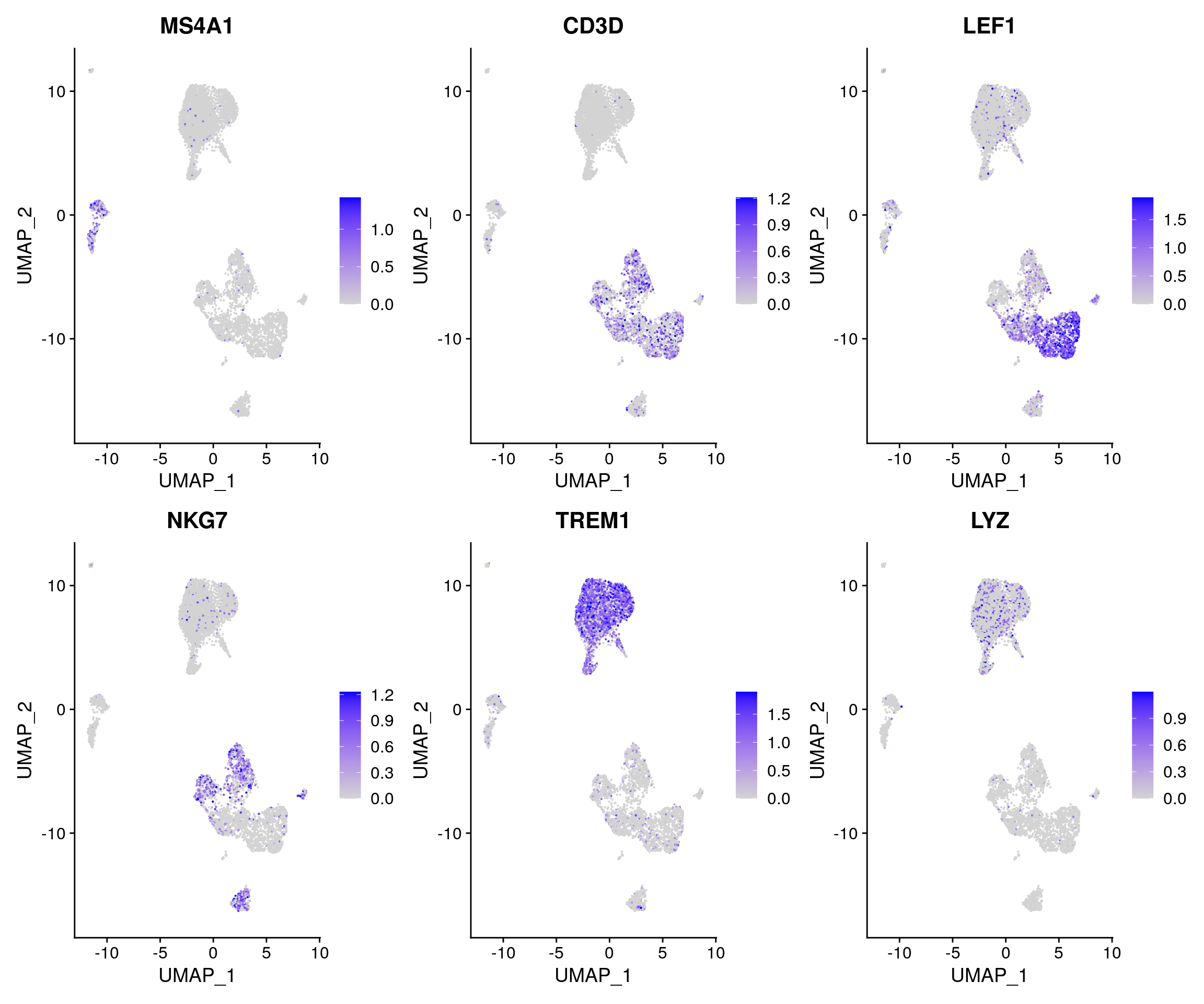
Now, we can visualize the ‘activities’ of canonical marker genes to help interpret our ATAC-seq clusters. Note that the activities will be much noisier than scRNA-seq measurements. This is because they represent predictions from sparse chromatin data, but also because they assume a general correspondence between gene body/promoter accessibility and expression, which may not always be the case. Nonetheless, we can begin to discern populations of monocytes, B, T, and NK cells. However, further subdivision of these cell types is challenging based on supervised analysis alone.
DefaultAssay(pbmc) <- 'RNA'

FeaturePlot(
  object = pbmc,
  features = c('MS4A1', 'CD3D', 'LEF1', 'NKG7', 'TREM1', 'LYZ'),
  pt.size = 0.1,
  max.cutoff = 'q95',
  ncol = 3
)
Integrating with scRNA-seq data
To help interpret the scATAC-seq data, we can classify cells based on an scRNA-seq experiment from the same biological system (human PBMC). We utilize methods for cross-modality integration and label transfer, described here, with a more in-depth tutorial here. We aim to identify shared correlation patterns in the gene activity matrix and scRNA-seq dataset in order to identify matched biological states across the two modalities. This procedure returns a classification score for each cell, based on each scRNA-seq defined cluster label. Here we load a pre-processed scRNA-seq dataset for human PBMCs, also provided by 10x Genomics. You can download the raw data for this experiment from the 10x website, and view the code used to construct this object on GitHub. Alternatively, you can download the pre-processed Seurat object here.
# Load the pre-processed scRNA-seq data for PBMCs
pbmc_rna <- readRDS("/home/stuartt/github/chrom/vignette_data/pbmc_10k_v3.rds")

transfer.anchors <- FindTransferAnchors(
  reference = pbmc_rna,
  query = pbmc,
  reduction = 'cca'
)

predicted.labels <- TransferData(
  anchorset = transfer.anchors,
  refdata = pbmc_rna$celltype,
  weight.reduction = pbmc[['lsi']],
  dims = 2:30
)

pbmc <- AddMetaData(object = pbmc, metadata = predicted.labels)
plot1 <- DimPlot(
  object = pbmc_rna,
  group.by = 'celltype',
  label = TRUE,
  repel = TRUE) + NoLegend() + ggtitle('scRNA-seq')

plot2 <- DimPlot(
  object = pbmc,
  group.by = 'predicted.id',
  label = TRUE,
  repel = TRUE) + NoLegend() + ggtitle('scATAC-seq')

plot1 + plot2
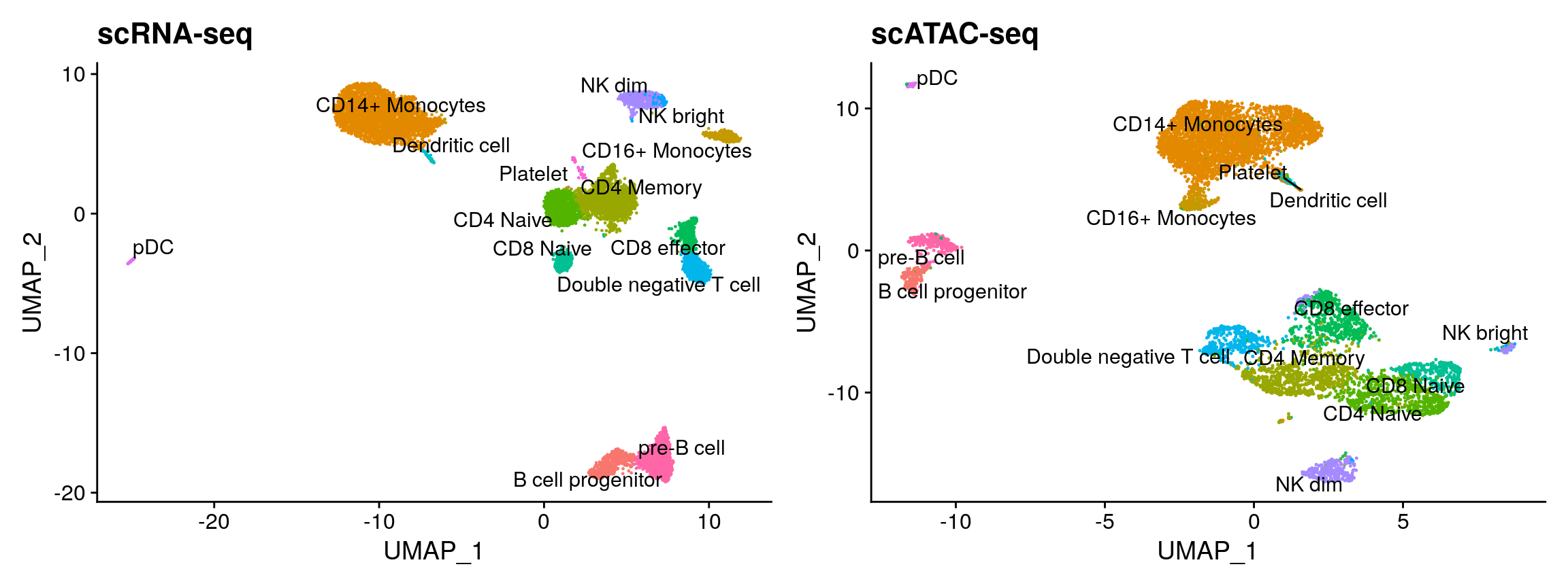
You can see that the RNA-based classifications are entirely consistent with the UMAP visualization, computed only on the ATAC-seq data. We can now easily annotate our scATAC-seq derived clusters (alternately, we could use the RNA classifications themselves). We note that cluster 14 maps to CD4 Memory T cells, but is a very small cluster with lower QC metrics. As this group is likely representing low-quality cells, we remove it from downstream analysis.
pbmc <- subset(pbmc,idents = 14, invert = TRUE)
pbmc <- RenameIdents(
  object = pbmc,
  '0' = 'CD14 Mono',
  '1' = 'CD4 Memory',
  '2' = 'CD8 Effector',
  '3' = 'CD4 Naive',
  '4' = 'CD14 Mono',
  '5' = 'CD8 Naive',
  '6' = 'DN T',
  '7' = 'NK CD56Dim',
  '8' = 'pre-B',
  '9' = 'CD16 Mono',
  '10' = 'pro-B',
  '11' = 'DC',
  '12' = 'NK CD56bright',
  '13' = 'pDC'
)
Find differentially accessible peaks between clusters
To find differentially accessible regions between clusters of cells, we can perform a differential accessibility (DA) test. We utilize logistic regression for DA, as suggested by Ntranos et al. 2018 for scRNA-seq data, and add the total number of fragments as a latent variable to mitigate the effect of differential sequencing depth on the result. Here we will focus on comparing Naive CD4 cells and CD14 monocytes, but any groups of cells can be compared using these methods. We can also visualize these chromatin ‘markers’ on a violin plot, feature plot, dot plot, heat map, or any visualization tool in Seurat.
# switch back to working with peaks instead of gene activities
DefaultAssay(pbmc) <- 'peaks'

da_peaks <- FindMarkers(
  object = pbmc,
  ident.1 = "CD4 Naive",
  ident.2 = "CD14 Mono",
  min.pct = 0.2,
  test.use = 'LR',
  latent.vars = 'peak_region_fragments'
)

head(da_peaks)
##                                  p_val  avg_logFC pct.1 pct.2     p_val_adj
## chr14:99721608-99741934   0.000000e+00  0.7882896 0.852 0.024  0.000000e+00
## chr7:142501666-142511108 5.528525e-272  0.7151732 0.747 0.031 4.937360e-267
## chr17:80084198-80086094  7.256824e-265  1.1305157 0.666 0.006 6.480852e-260
## chr14:99695477-99720910  4.629419e-261  0.7638794 0.778 0.023 4.134396e-256
## chr2:113581628-113594911 2.977877e-243 -0.8919683 0.049 0.693 2.659453e-238
## chr6:44025105-44028184   6.532939e-231 -0.8710842 0.057 0.655 5.834372e-226
plot1 <- VlnPlot( object = pbmc, features = rownames(da_peaks)[1], pt.size = 0.1, idents = c("CD4 Memory","CD14 Mono") ) plot2 <- FeaturePlot( object = pbmc, features = rownames(da_peaks)[1], pt.size = 0.1 ) plot1 | plot2
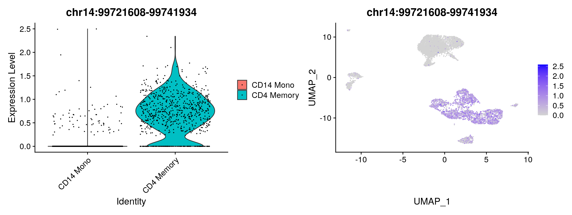
Peak coordinates can be difficult to interpret alone. We can find the closest gene to each of these peaks using the ClosestFeature function and providing an EnsDb annotation. If you explore the gene lists, you will see that peaks open in Naive T cells are close to genes such as BCL11B and GATA3 (key regulator of T cell differentiation), while peaks open in monocytes are close to genes such as CEBPB (key regulator of monocyte differentiation). We could follow up this result further by doing gene ontology enrichment analysis on the gene sets returned by ClosestFeature, and there are many R packages that can do this (see the GOstats package for example).
open_cd4naive <- rownames(da_peaks[da_peaks$avg_logFC > 0.5, ])
open_cd14mono <- rownames(da_peaks[da_peaks$avg_logFC < -0.5, ])

closest_genes_cd4naive <- ClosestFeature(
  regions = open_cd4naive,
  annotation = gene.ranges,
  sep = c(':', '-')
)
closest_genes_cd14mono <- ClosestFeature(
  regions = open_cd14mono,
  annotation = gene.ranges,
  sep = c(':', '-')
)
head(closest_genes_cd4naive)
##                           gene_id gene_name   gene_biotype seq_coord_system
## ENSG00000127152   ENSG00000127152    BCL11B protein_coding       chromosome
## ENSG00000204983   ENSG00000204983     PRSS1 protein_coding       chromosome
## ENSG00000176155   ENSG00000176155    CCDC57 protein_coding       chromosome
## ENSG00000127152.1 ENSG00000127152    BCL11B protein_coding       chromosome
## ENSG00000134709   ENSG00000134709     HOOK1 protein_coding       chromosome
## ENSG00000134954   ENSG00000134954      ETS1 protein_coding       chromosome
##                   symbol   entrezid            closest_region
## ENSG00000127152   BCL11B      64919   chr14:99635624-99737861
## ENSG00000204983    PRSS1 5645, 5644  chr7:142457319-142460923
## ENSG00000176155   CCDC57     284001   chr17:80059336-80170706
## ENSG00000127152.1 BCL11B      64919   chr14:99635624-99737861
## ENSG00000134709    HOOK1      51361    chr1:60280458-60342050
## ENSG00000134954     ETS1       2113 chr11:128328656-128457453
##                                query_region distance
## ENSG00000127152     chr14:99721608-99741934        0
## ENSG00000204983    chr7:142501666-142511108    40742
## ENSG00000176155     chr17:80084198-80086094        0
## ENSG00000127152.1   chr14:99695477-99720910        0
## ENSG00000134709      chr1:60279767-60281364        0
## ENSG00000134954 chr11:128334097-128348572 0head(closest_genes_cd14mono)
## gene_id gene_name gene_biotype seq_coord_system
## ENSG00000125538 ENSG00000125538 IL1B protein_coding chromosome
## ENSG00000181577 ENSG00000181577 C6orf223 protein_coding chromosome
## ENSG00000172216 ENSG00000172216 CEBPB protein_coding chromosome
## ENSG00000138621 ENSG00000138621 PPCDC protein_coding chromosome
## ENSG00000273269 ENSG00000273269 RP11-761B3.1 protein_coding chromosome
## ENSG00000186350 ENSG00000186350 RXRA protein_coding chromosome
## symbol entrezid closest_region
## ENSG00000125538 IL1B 3553 chr2:113587328-113594480
## ENSG00000181577 C6orf223 221416 chr6:43968317-43973695
## ENSG00000172216 CEBPB 1051 chr20:48807376-48809212
## ENSG00000138621 PPCDC 60490 chr15:75315896-75409803
## ENSG00000273269 RP11-761B3.1 NA chr2:47293080-47403650
## ENSG00000186350 RXRA 6256 chr9:137208944-137332431
## query_region distance
## ENSG00000125538 chr2:113581628-113594911 0
## ENSG00000181577 chr6:44025105-44028184 51409
## ENSG00000172216 chr20:48889794-48893313 80581
## ENSG00000138621 chr15:75334903-75336779 0
## ENSG00000273269 chr2:47297968-47301173 0
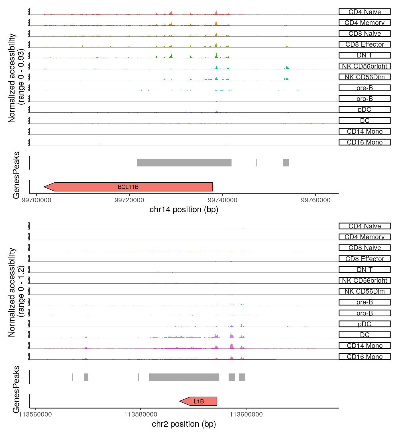
## ENSG00000186350 chr9:137263243-137268534 0We can also create coverage plots grouped by cluster around any genomic region using the CoveragePlot function. These represent ‘pseudo-bulk’ accessibility tracks, where all cells within a cluster have been averaged together, in order to visualize a more robust chromatin landscape (thanks to Andrew Hill for giving the inspiration for this function in his excellent blog post).
# set plotting order
levels(pbmc) <- c("CD4 Naive","CD4 Memory","CD8 Naive","CD8 Effector","DN T","NK CD56bright","NK CD56Dim","pre-B",'pro-B',"pDC","DC","CD14 Mono",'CD16 Mono')

CoveragePlot(
  object = pbmc,
  region = rownames(da_peaks)[c(1,5)],
  sep = c(":", "-"),
  peaks = StringToGRanges(rownames(pbmc), sep = c(":", "-")),
  annotation = gene.ranges,
  extend.upstream = 20000,
  extend.downstream = 20000,
  ncol = 1
)
Working with datasets that were not quantified using CellRanger
The CellRanger software from 10x Genomics generates several useful QC metrics per-cell, as well as a peak/cell matrix and an indexed fragments file. In the above vignette, we utilize the CellRanger outputs, but provide alternative functions in Signac for many of the same purposes here.
Generating a peak/cell or bin/cell matrix
The FeatureMatrix function can be used to generate a count matrix containing any set of genomic ranges in its rows. These regions could be a set of peaks, or bins that span the entire genome.
# not run
# peak_ranges should be a set of genomic ranges spanning the set of peaks to be quantified per cell
peak_matrix <- FeatureMatrix(
  fragments = fragment.path,
  features = peak_ranges
)
For convenience, we also include a GenomeBinMatrix function that will generate a set of genomic ranges spanning the entire genome for you, and run FeatureMatrix internally to produce a genome bin/cell matrix.
# not run
bin_matrix <- GenomeBinMatrix(
  fragments = fragment.path,
  genome = 'hg19',
  binsize = 5000
)
Counting fraction of reads in peaks
The function FRiP will count the fraction of reads in peaks for each cell, given a peak/cell assay and a bin/cell assay. Note that this can be run on a subset of the genome, so that a bin/cell assay does not need to be computed for the whole genome. This will return a Seurat object will metadata added corresponding to the fraction of reads in peaks for each cell.
# not run
pbmc <- FRiP(
  object = pbmc,
  peak.assay = 'peaks',
  bin.assay = 'bins'
)
Counting fragments in genome blacklist regions
The ratio of reads in genomic blacklist regions, that are known to artifactually accumulate reads in genome sequencing assays, can be diagnostic of low-quality cells. We provide blacklist region coordinates for several genomes (hg19, hg38, mm9, mm10, ce10, ce11, dm3, dm6) in the Signac package for convenience. These regions were provided by the ENCODE consortium, and we encourage users to cite their paper if you use the regions in your analysis. The FractionCountsInRegion function can be used to calculate the fraction of all counts within a given set of regions per cell. We can use this function and the blacklist regions to find the fraction of blacklist counts per cell.
# not run
pbmc$blacklist_fraction <- FractionCountsInRegion(
  object = pbmc,
  assay = 'peaks',
  regions = blacklist_hg19
)
Session Info
## R version 4.0.1 (2020-06-06)
## Platform: x86_64-pc-linux-gnu (64-bit)
## Running under: Ubuntu 18.04.4 LTS
##
## Matrix products: default
## BLAS:   /usr/lib/x86_64-linux-gnu/blas/libblas.so.3.7.1
## LAPACK: /usr/lib/x86_64-linux-gnu/lapack/liblapack.so.3.7.1
##
## locale:
##  [1] LC_CTYPE=en_AU.UTF-8       LC_NUMERIC=C
##  [3] LC_TIME=en_US.UTF-8        LC_COLLATE=en_US.UTF-8
##  [5] LC_MONETARY=en_US.UTF-8    LC_MESSAGES=en_US.UTF-8
##  [7] LC_PAPER=en_US.UTF-8       LC_NAME=C
##  [9] LC_ADDRESS=C               LC_TELEPHONE=C
## [11] LC_MEASUREMENT=en_US.UTF-8 LC_IDENTIFICATION=C
##
## attached base packages:
## [1] stats4    parallel  stats     graphics  grDevices utils     datasets
## [8] methods   base
##
## other attached packages:
##  [1] dplyr_1.0.0               patchwork_1.0.1
##  [3] ggplot2_3.3.2             EnsDb.Hsapiens.v75_2.99.0
##  [5] ensembldb_2.12.1          AnnotationFilter_1.12.0
##  [7] GenomicFeatures_1.40.0    AnnotationDbi_1.50.0
##  [9] Biobase_2.48.0            GenomicRanges_1.40.0
## [11] GenomeInfoDb_1.24.0       IRanges_2.22.2
## [13] S4Vectors_0.26.1          BiocGenerics_0.34.0
## [15] Seurat_3.1.5.9009         Signac_0.2.5
##
## loaded via a namespace (and not attached):
##   [1] backports_1.1.8             BiocFileCache_1.12.0
##   [3] plyr_1.8.6                  igraph_1.2.5
##   [5] lazyeval_0.2.2              splines_4.0.1
##   [7] BiocParallel_1.22.0         listenv_0.8.0
##   [9] digest_0.6.25               htmltools_0.5.0
##  [11] magrittr_1.5                memoise_1.1.0
##  [13] cluster_2.1.0               ROCR_1.0-11
##  [15] globals_0.12.5              Biostrings_2.56.0
##  [17] ggfittext_0.9.0             matrixStats_0.56.0
##  [19] askpass_1.1                 pkgdown_1.5.1
##  [21] prettyunits_1.1.1           colorspace_1.4-1
##  [23] blob_1.2.1                  rappdirs_0.3.1
##  [25] ggrepel_0.8.2               xfun_0.14
##  [27] crayon_1.3.4                RCurl_1.98-1.2
##  [29] jsonlite_1.7.0              survival_3.2-3
##  [31] zoo_1.8-8                   ape_5.4
##  [33] glue_1.4.1                  gtable_0.3.0
##  [35] zlibbioc_1.34.0             XVector_0.28.0
##  [37] leiden_0.3.3                DelayedArray_0.14.0
##  [39] future.apply_1.6.0          scales_1.1.1
##  [41] DBI_1.1.0                   Rcpp_1.0.5
##  [43] viridisLite_0.3.0           progress_1.2.2
##  [45] reticulate_1.16             bit_1.1-15.2
##  [47] rsvd_1.0.3                  htmlwidgets_1.5.1
##  [49] httr_1.4.1                  RColorBrewer_1.1-2
##  [51] ellipsis_0.3.1              ica_1.0-2
##  [53] farver_2.0.3                pkgconfig_2.0.3
##  [55] XML_3.99-0.3                ggseqlogo_0.1
##  [57] uwot_0.1.8                  dbplyr_1.4.4
##  [59] labeling_0.3                tidyselect_1.1.0
##  [61] rlang_0.4.6                 reshape2_1.4.4
##  [63] munsell_0.5.0               tools_4.0.1
##  [65] generics_0.0.2              RSQLite_2.2.0
##  [67] ggridges_0.5.2              evaluate_0.14
##  [69] stringr_1.4.0               yaml_2.2.1
##  [71] knitr_1.28                  bit64_0.9-7
##  [73] fs_1.4.1                    fitdistrplus_1.1-1
##  [75] purrr_0.3.4                 RANN_2.6.1
##  [77] pbapply_1.4-2               future_1.17.0
##  [79] nlme_3.1-148                biomaRt_2.44.0
##  [81] hdf5r_1.3.2                 compiler_4.0.1
##  [83] plotly_4.9.2.1              curl_4.3
##  [85] png_0.1-7                   tibble_3.0.1
##  [87] stringi_1.4.6               desc_1.2.0
##  [89] lattice_0.20-41             ProtGenerics_1.20.0
##  [91] Matrix_1.2-18               vctrs_0.3.1
##  [93] pillar_1.4.4                lifecycle_0.2.0
##  [95] lmtest_0.9-37               RcppAnnoy_0.0.16
##  [97] data.table_1.12.8           cowplot_1.0.0
##  [99] bitops_1.0-6                irlba_2.3.3
## [101] gggenes_0.4.0               rtracklayer_1.48.0
## [103] R6_2.4.1                    KernSmooth_2.23-17
## [105] gridExtra_2.3               codetools_0.2-16
## [107] MASS_7.3-51.6               assertthat_0.2.1
## [109] SummarizedExperiment_1.18.1 openssl_1.4.2
## [111] rprojroot_1.3-2             withr_2.2.0
## [113] GenomicAlignments_1.24.0    sctransform_0.2.1
## [115] Rsamtools_2.4.0             GenomeInfoDbData_1.2.3
## [117] hms_0.5.3                   grid_4.0.1
## [119] tidyr_1.1.0                 rmarkdown_2.2
## [121] Rtsne_0.15