When merging multiple single-cell chromatin datasets, it’s important to be aware that if peak calling was performed on each dataset independently, the peaks are unlikely to perfectly overlap. Any peaks that are not exactly the same are treated as different features by Seurat. Therefore, we need to create a common set of peaks across all the datasets to be merged.
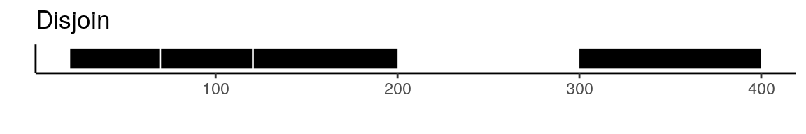
To create a unified set of peaks we can use functions from the GenomicRanges package. The reduce function from GenomicRanges will merge all intersecting peaks. Another option is to use the disjoin function, that will create distinct non-overlapping sets of peaks. Here is a visual example to illustrate the difference between reduce and disjoin:
gr <- GRanges(seqnames = "chr1", ranges = IRanges(start = c(20, 70, 300), end = c(120, 200, 400)))
gr
## GRanges object with 3 ranges and 0 metadata columns:
##       seqnames    ranges strand
##          <Rle> <IRanges>  <Rle>
##   [1]     chr1    20-120      *
##   [2]     chr1    70-200      *
##   [3]     chr1   300-400      *
##   -------
##   seqinfo: 1 sequence from an unspecified genome; no seqlengths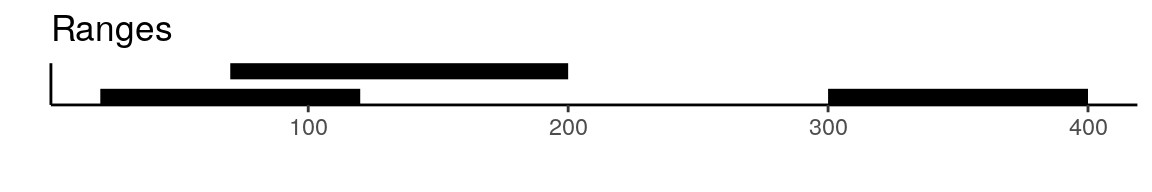

Alternatively, we can treat overlapping peaks as equivalent, and rename peaks that overlap with a common name so that they are recognized as equivalent by Seurat. This is what is done by the MergeWithRegions function. See the See the integration vignette for a demonstration of the MergeWithRegions function.
In this vignette we demonstrate how to merge multiple Seurat objects containing single-cell chromatin data, by creating a new assay in each object containing a common set of peaks.
To demonstrate, we will use four scATAC-seq PBMC datasets provided by 10x Genomics:
Loading data
# define a convenient function to load all the data and create a Seurat object
create_obj <- function(dir) {
  count.path <- list.files(path = dir, pattern = "*_filtered_peak_bc_matrix.h5", full.names = TRUE)
  fragment.path <- list.files(path = dir, pattern = "*_fragments.tsv.gz", full.names = TRUE)[1]
  counts <- Read10X_h5(count.path)
  md.path <- list.files(path = dir, pattern = "*_singlecell.csv", full.names = TRUE)
  md <- read.table(file = md.path, stringsAsFactors = FALSE, sep = ",", header = TRUE, row.names = 1)
  obj <- CreateSeuratObject(counts = counts, assay = "ATAC", meta.data = md)
  obj <- SetFragments(obj, file = fragment.path)
  return(obj)
}
pbmc500 <- create_obj("/home/stuartt/data/pbmc500")
pbmc1k <- create_obj("/home/stuartt/data/pbmc1k")
pbmc5k <- create_obj("/home/stuartt/data/pbmc5k")
pbmc10k <- create_obj("/home/stuartt/data/pbmc10k")
After creating each object, we can perform standard pre-processing and quality control on each object as shown in other vignettes. For brevity, we will skip this step here and proceed with merging the objects.
Creating a common peak set
If the peaks were identified independently in each experiment then they will likely not overlap perfectly. We can merge peaks from all the datasets to create a common peak set, and quantify this peak set in each experiment prior to merging the objects.
There are a few different ways that we can create a common peak set. One possibility is using the reduce or disjoin functions from the GenomicRanges package. The UnifyPeaks function extracts the peak coordinates from a list of objects and applies reduce or disjoin to the peak sets to create a single non-overlapping set of peaks.
combined.peaks <- UnifyPeaks(object.list = list(pbmc500, pbmc1k, pbmc5k, pbmc10k), mode = "reduce")
combined.peaks
## GRanges object with 90694 ranges and 0 metadata columns:
##           seqnames            ranges strand
##              <Rle>         <IRanges>  <Rle>
##       [1]     chr1     565153-565499      *
##       [2]     chr1     569185-569620      *
##       [3]     chr1     713551-714783      *
##       [4]     chr1     752418-753020      *
##       [5]     chr1     762249-763345      *
##       ...      ...               ...    ...
##   [90690]     chrY 23583994-23584463      *
##   [90691]     chrY 23602466-23602779      *
##   [90692]     chrY 23899155-23899164      *
##   [90693]     chrY 28816593-28817710      *
##   [90694]     chrY 58855911-58856251      *
##   -------
##   seqinfo: 24 sequences from an unspecified genome; no seqlengths
Quantify peaks in each dataset
We can now add a new assay to each object that contains counts for the same set of peaks. This will ensure that all the objects contain common features that we can use to merge the objects.
pbmc500.counts <- FeatureMatrix(
  fragments = GetFragments(pbmc500),
  features = combined.peaks,
  sep = c(":", "-"),
  cells = colnames(pbmc500)
)

pbmc1k.counts <- FeatureMatrix(
  fragments = GetFragments(pbmc1k),
  features = combined.peaks,
  sep = c(":", "-"),
  cells = colnames(pbmc1k)
)

pbmc5k.counts <- FeatureMatrix(
  fragments = GetFragments(pbmc5k),
  features = combined.peaks,
  sep = c(":", "-"),
  cells = colnames(pbmc5k)
)

pbmc10k.counts <- FeatureMatrix(
  fragments = GetFragments(pbmc10k),
  features = combined.peaks,
  sep = c(":", "-"),
  cells = colnames(pbmc10k)
)
pbmc500[['peaks']] <- CreateAssayObject(counts = pbmc500.counts)
pbmc1k[['peaks']] <- CreateAssayObject(counts = pbmc1k.counts)
pbmc5k[['peaks']] <- CreateAssayObject(counts = pbmc5k.counts)
pbmc10k[['peaks']] <- CreateAssayObject(counts = pbmc10k.counts)
Merge objects
Now that the objects each contain an assay with the same set of features, we can use the standard merge function from Seurat to merge the objects.
# add information to identify dataset of origin
pbmc500$dataset <- 'pbmc500'
pbmc1k$dataset <- 'pbmc1k'
pbmc5k$dataset <- 'pbmc5k'
pbmc10k$dataset <- 'pbmc10k'

# merge all datasets, adding a cell ID to make sure cell names are unique
combined <- merge(x = pbmc500, y = list(pbmc1k, pbmc5k, pbmc10k), add.cell.ids = c("500", "1k", "5k", "10k"))
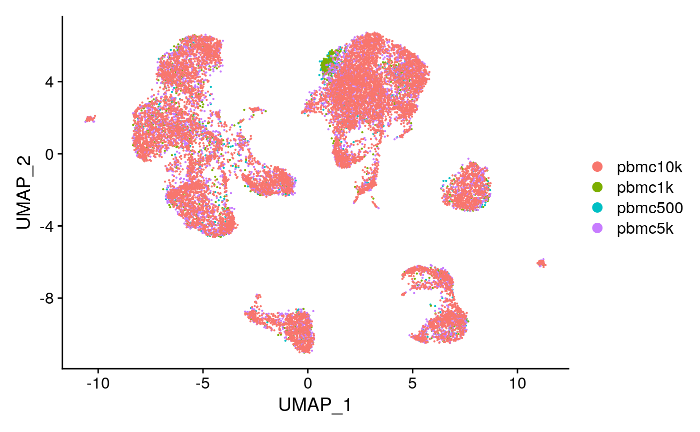
# make sure to change to the assay containing common peaks
DefaultAssay(combined) <- "peaks"
combined <- RunTFIDF(combined)
combined <- FindTopFeatures(combined, min.cutoff = 20)
combined <- RunSVD(
  combined,
  reduction.key = 'LSI_',
  reduction.name = 'lsi',
  irlba.work = 400
)
combined <- RunUMAP(combined, dims = 2:30, reduction = 'lsi')
DimPlot(combined, group.by = 'dataset', pt.size = 0.1)
At this stage it is possible to proceed with all downstream analysis without creating a merged fragment file if you have computed quality control metrics and gene activities for each object individually prior to merging the datasets, and don’t need to plot coverage tracks with the merged data.
If you need to construct a merged fragment file, we demonstrate how to do this below.
Merge fragment files
To create a merged fragment file we need to decompress the files, add the same cell ID that was added to the cell barcodes in the Seurat object, merge the files, and finally compress and index the merged file. This is performed on the command line rather than in R.
Note that the workflow is the same for any number of datasets. Commands such as gzip, bgzip, and sort can take any number of input files.
You will need to make sure tabix and bgzip are installed.
# decompress files and add the same cell prefix as was added to the Seurat object
gzip -dc atac_pbmc_500_nextgem_fragments.tsv.gz | awk 'BEGIN {FS=OFS="\t"} {print $1,$2,$3,"500_"$4,$5}' - > pbmc500_fragments.tsv
gzip -dc atac_pbmc_1k_nextgem_fragments.tsv.gz | awk 'BEGIN {FS=OFS="\t"} {print $1,$2,$3,"1k_"$4,$5}' - > pbmc1k_fragments.tsv
gzip -dc atac_pbmc_5k_nextgem_fragments.tsv.gz | awk 'BEGIN {FS=OFS="\t"} {print $1,$2,$3,"5k_"$4,$5}' - > pbmc5k_fragments.tsv
gzip -dc atac_pbmc_10k_nextgem_fragments.tsv.gz | awk 'BEGIN {FS=OFS="\t"} {print $1,$2,$3,"10k_"$4,$5}' - > pbmc10k_fragments.tsv

# merge files (avoids having to re-sort)
sort -m -k 1,1V -k2,2n pbmc500_fragments.tsv pbmc1k_fragments.tsv pbmc5k_fragments.tsv pbmc10k_fragments.tsv > fragments.tsv

# block gzip compress the merged file
bgzip -@ 4 fragments.tsv # -@ 4 uses 4 threads

# index the bgzipped file
tabix -p bed fragments.tsv.gz

# remove intermediate files
rm pbmc500_fragments.tsv pbmc1k_fragments.tsv pbmc5k_fragments.tsv pbmc10k_fragments.tsv
We can now add the path to the merged fragment file to the Seurat object:
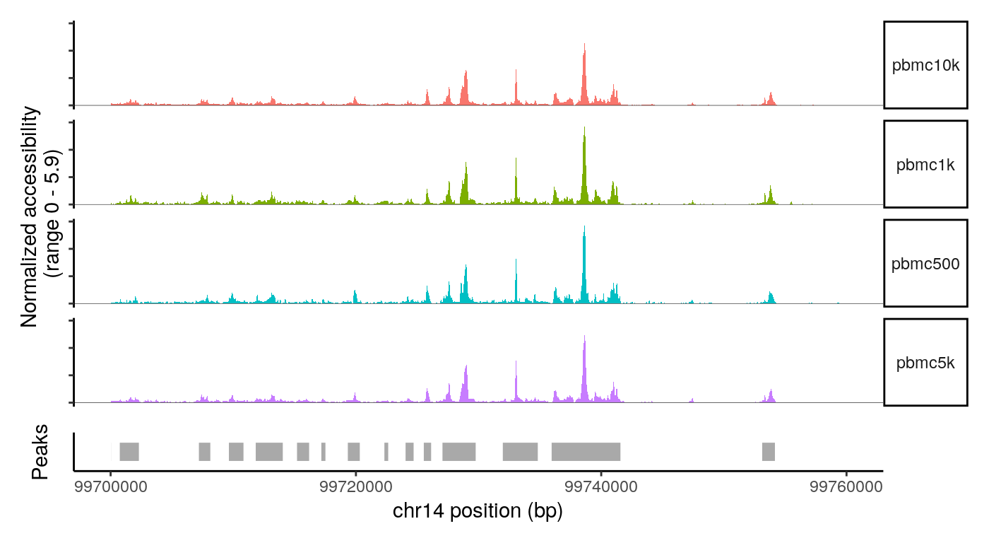
combined <- SetFragments(combined, "/home/stuartt/data/pbmc_combined/fragments.tsv.gz")
CoveragePlot(
  object = combined,
  group.by = 'dataset',
  region = "chr14-99700000-99760000",
  peaks = StringToGRanges(rownames(combined), sep = c(":", "-"))
)
Session Info
## R version 4.0.1 (2020-06-06)
## Platform: x86_64-pc-linux-gnu (64-bit)
## Running under: Ubuntu 18.04.4 LTS
##
## Matrix products: default
## BLAS:   /usr/lib/x86_64-linux-gnu/blas/libblas.so.3.7.1
## LAPACK: /usr/lib/x86_64-linux-gnu/lapack/liblapack.so.3.7.1
##
## locale:
##  [1] LC_CTYPE=en_AU.UTF-8       LC_NUMERIC=C
##  [3] LC_TIME=en_US.UTF-8        LC_COLLATE=en_US.UTF-8
##  [5] LC_MONETARY=en_US.UTF-8    LC_MESSAGES=en_US.UTF-8
##  [7] LC_PAPER=en_US.UTF-8       LC_NAME=C
##  [9] LC_ADDRESS=C               LC_TELEPHONE=C
## [11] LC_MEASUREMENT=en_US.UTF-8 LC_IDENTIFICATION=C
##
## attached base packages:
## [1] parallel  stats4    stats     graphics  grDevices utils     datasets
## [8] methods   base
##
## other attached packages:
##  [1] Seurat_3.1.5.9009    Signac_0.2.5         patchwork_1.0.1
##  [4] ggbio_1.36.0         ggplot2_3.3.2        GenomicRanges_1.40.0
##  [7] GenomeInfoDb_1.24.0  IRanges_2.22.2       S4Vectors_0.26.1
## [10] BiocGenerics_0.34.0
##
## loaded via a namespace (and not attached):
##   [1] backports_1.1.8             Hmisc_4.4-0
##   [3] BiocFileCache_1.12.0        plyr_1.8.6
##   [5] igraph_1.2.5                lazyeval_0.2.2
##   [7] splines_4.0.1               BiocParallel_1.22.0
##   [9] listenv_0.8.0               digest_0.6.25
##  [11] ensembldb_2.12.1            htmltools_0.5.0
##  [13] magrittr_1.5                checkmate_2.0.0
##  [15] memoise_1.1.0               BSgenome_1.56.0
##  [17] cluster_2.1.0               ROCR_1.0-11
##  [19] ggfittext_0.9.0             globals_0.12.5
##  [21] Biostrings_2.56.0           matrixStats_0.56.0
##  [23] askpass_1.1                 pkgdown_1.5.1
##  [25] prettyunits_1.1.1           jpeg_0.1-8.1
##  [27] colorspace_1.4-1            blob_1.2.1
##  [29] rappdirs_0.3.1              ggrepel_0.8.2
##  [31] xfun_0.14                   dplyr_1.0.0
##  [33] jsonlite_1.7.0              crayon_1.3.4
##  [35] RCurl_1.98-1.2              graph_1.66.0
##  [37] zoo_1.8-8                   survival_3.2-3
##  [39] VariantAnnotation_1.34.0    ape_5.4
##  [41] glue_1.4.1                  gtable_0.3.0
##  [43] zlibbioc_1.34.0             XVector_0.28.0
##  [45] leiden_0.3.3                DelayedArray_0.14.0
##  [47] future.apply_1.6.0          scales_1.1.1
##  [49] DBI_1.1.0                   GGally_2.0.0
##  [51] Rcpp_1.0.5                  viridisLite_0.3.0
##  [53] progress_1.2.2              htmlTable_1.13.3
##  [55] reticulate_1.16             rsvd_1.0.3
##  [57] foreign_0.8-80              bit_1.1-15.2
##  [59] OrganismDbi_1.30.0          Formula_1.2-3
##  [61] htmlwidgets_1.5.1           httr_1.4.1
##  [63] RColorBrewer_1.1-2          acepack_1.4.1
##  [65] ellipsis_0.3.1              ica_1.0-2
##  [67] pkgconfig_2.0.3             reshape_0.8.8
##  [69] XML_3.99-0.3                farver_2.0.3
##  [71] ggseqlogo_0.1               uwot_0.1.8
##  [73] nnet_7.3-14                 dbplyr_1.4.4
##  [75] tidyselect_1.1.0            labeling_0.3
##  [77] rlang_0.4.6                 reshape2_1.4.4
##  [79] AnnotationDbi_1.50.0        munsell_0.5.0
##  [81] tools_4.0.1                 generics_0.0.2
##  [83] RSQLite_2.2.0               ggridges_0.5.2
##  [85] evaluate_0.14               stringr_1.4.0
##  [87] yaml_2.2.1                  knitr_1.28
##  [89] bit64_0.9-7                 fs_1.4.1
##  [91] fitdistrplus_1.1-1          purrr_0.3.4
##  [93] RANN_2.6.1                  AnnotationFilter_1.12.0
##  [95] pbapply_1.4-2               RBGL_1.64.0
##  [97] future_1.17.0               nlme_3.1-148
##  [99] biomaRt_2.44.0              hdf5r_1.3.2
## [101] compiler_4.0.1              rstudioapi_0.11
## [103] plotly_4.9.2.1              curl_4.3
## [105] png_0.1-7                   tibble_3.0.1
## [107] stringi_1.4.6               GenomicFeatures_1.40.0
## [109] desc_1.2.0                  lattice_0.20-41
## [111] ProtGenerics_1.20.0         Matrix_1.2-18
## [113] vctrs_0.3.1                 pillar_1.4.4
## [115] lifecycle_0.2.0             BiocManager_1.30.10
## [117] lmtest_0.9-37               RcppAnnoy_0.0.16
## [119] data.table_1.12.8           cowplot_1.0.0
## [121] bitops_1.0-6                irlba_2.3.3
## [123] gggenes_0.4.0               rtracklayer_1.48.0
## [125] R6_2.4.1                    latticeExtra_0.6-29
## [127] KernSmooth_2.23-17          gridExtra_2.3
## [129] codetools_0.2-16            dichromat_2.0-0
## [131] MASS_7.3-51.6               assertthat_0.2.1
## [133] SummarizedExperiment_1.18.1 openssl_1.4.2
## [135] rprojroot_1.3-2             withr_2.2.0
## [137] sctransform_0.2.1           GenomicAlignments_1.24.0
## [139] Rsamtools_2.4.0             GenomeInfoDbData_1.2.3
## [141] hms_0.5.3                   grid_4.0.1
## [143] rpart_4.1-15                tidyr_1.1.0
## [145] rmarkdown_2.2               Rtsne_0.15
## [147] biovizBase_1.36.0           Biobase_2.48.0
## [149] base64enc_0.1-3