Here we demonstrate the integration of multiple single-cell ATAC-seq datasets from the adult mouse brain, profiled using 10x Genomics and sci-ATAC-seq. The dataset from 10x Genomics is the same as used in our mouse brain vignette, and you can find links to download the raw data as well as the code used to produce the processed Seurat object used in this vignette on the mouse brain vignette page.
The sci-ATAC-seq dataset was generated by Cusanovich and Hill et al.. Raw data can be downloaded from the authors’ website:
We will demonstrate the use of Seurat v3 integration methods described here on scATAC-seq data, for both dataset integration and label transfer between datasets, as well as use of the harmony package for dataset integration.
First, we load the required packages, read in the data and create a Seurat object for the sci-ATAC-seq data.
Preprocessing
library(Signac)
library(Seurat)
library(patchwork)
set.seed(1234)

# this object was created following the mouse brain vignette
tenx <- readRDS(file = "../vignette_data/adult_mouse_brain.rds")
tenx$tech <- '10x'
tenx$celltype <- Idents(tenx)

sci.metadata <- read.table(
  file = "../vignette_data/sci/cell_metadata.txt",
  header = TRUE,
  row.names = 1,
  sep = "\t"
)
# subset to include only the brain data
sci.metadata <- sci.metadata[sci.metadata$tissue == 'PreFrontalCortex', ]
sci.counts <- readRDS(file = "../vignette_data/sci/atac_matrix.binary.qc_filtered.rds")
sci.counts <- sci.counts[, rownames(x = sci.metadata)]
The sci-ATAC-seq data was mapped to the mm9 mouse genome, whereas the 10x data was mapped to mm10, and so the coordinate space of the peaks in each experiment are different. We can lift over the mm9 coordinates to mm10 using the rtracklayer package, and rename the sci-ATAC-seq peaks with mm10 coordinates. Liftover chains can be downloaded from UCSC. See this post on biostars for more information about lifting over genomic coordinates.
sci_peaks_mm9 <- StringToGRanges(regions = rownames(sci.counts), sep = c("_", "_"))
mm9_mm10 <- rtracklayer::import.chain("/home/stuartt/data/liftover/mm9ToMm10.over.chain")
sci_peaks_mm10 <- rtracklayer::liftOver(x = sci_peaks_mm9, chain = mm9_mm10)
names(sci_peaks_mm10) <- rownames(sci.counts)

# discard any peaks that were mapped to >1 region in mm10
correspondence <- S4Vectors::elementNROWS(sci_peaks_mm10)
sci_peaks_mm10 <- sci_peaks_mm10[correspondence == 1]
sci_peaks_mm10 <- unlist(sci_peaks_mm10)
sci.counts <- sci.counts[names(sci_peaks_mm10), ]

# rename peaks with mm10 coordinates
rownames(sci.counts) <- GRangesToString(grange = sci_peaks_mm10)

# create Seurat object and perform some basic QC filtering
sci <- CreateSeuratObject(
  counts = sci.counts,
  meta.data = sci.metadata,
  assay = 'peaks',
  project = 'sci'
)
sci.ds <- sci[, sci$nFeature_peaks > 2000 & sci$nCount_peaks > 5000 & !(sci$cell_label %in% c("Collisions", "Unknown"))]
sci$tech <- 'sciATAC'
sci <- RunTFIDF(sci)
sci <- FindTopFeatures(sci, min.cutoff = 50)
sci <- RunSVD(sci, n = 30, reduction.name = 'lsi', reduction.key = 'LSI_')
sci <- RunUMAP(sci, reduction = 'lsi', dims = 2:30)
We now have two scATAC-seq objects containing features in a common coordinate space. However, as the peak calling was performed independently in each experiment, it is unlikely that the peak coordinates overlap perfectly. In order to have common features across the datasets we want to integrate, we can count reads in the sci-ATAC-seq peaks in the 10x Genomics dataset and create a new assay with these counts. For efficiency, we will downsample the sci-ATAC-seq peaks used. We have found integration results to be quite robust to the number and set of peaks used.
# find peaks that intersect in both datasets
intersecting.regions <- GetIntersectingFeatures(
  object.1 = sci,
  object.2 = tenx,
  sep.1 = c("-", "-"),
  sep.2 = c(":", "-")
)

# choose a subset of intersecting peaks
peaks.use <- sample(intersecting.regions[[1]], size = 10000, replace = FALSE)

# count fragments per cell overlapping the set of peaks in the 10x data
sci_peaks_tenx <- FeatureMatrix(
  fragments = GetFragments(object = tenx, assay = 'peaks'),
  features = StringToGRanges(peaks.use),
  cells = colnames(tenx)
)

# create a new assay and add it to the 10x dataset
tenx[['sciPeaks']] <- CreateAssayObject(counts = sci_peaks_tenx, min.cells = 1)
tenx <- RunTFIDF(object = tenx, assay = 'sciPeaks')
Integration
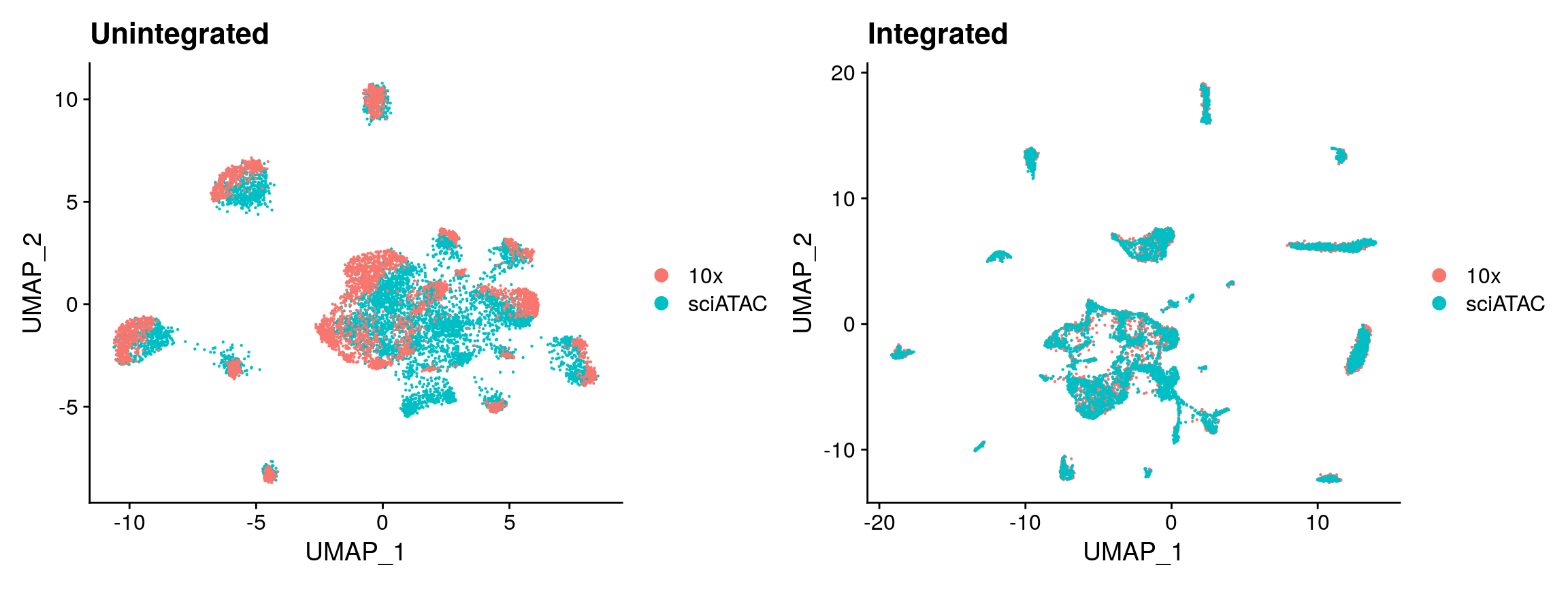
Before performing integration it is always a good idea to check if there are dataset-specific difference present that need to be removed. If not, we could simply merge the objects without performing integration. In this case there is a strong difference between the two datasets due to the different technologies used. This effect can be removed using the integration methods in Seurat v3 described in this paper.
# Look at the data without integration first
unintegrated <- MergeWithRegions(
  object.1 = sci,
  object.2 = tenx,
  assay.1 = 'peaks',
  assay.2 = 'sciPeaks',
  sep.1 = c("-", "-"),
  sep.2 = c("-", "-")
)

unintegrated <- RunTFIDF(unintegrated)
unintegrated <- FindTopFeatures(unintegrated, min.cutoff = 50)
unintegrated <- RunSVD(unintegrated, n = 30, reduction.name = 'lsi', reduction.key = 'LSI_')
unintegrated <- RunUMAP(unintegrated, reduction = 'lsi', dims = 2:30)
p1 <- DimPlot(unintegrated, group.by = 'tech', pt.size = 0.1) + ggplot2::ggtitle("Unintegrated")

# find integration anchors between 10x and sci-ATAC
anchors <- FindIntegrationAnchors(
  object.list = list(tenx, sci),
  anchor.features = peaks.use,
  assay = c('sciPeaks', 'peaks'),
  k.filter = NA
)

# integrate data and create a new merged object
integrated <- IntegrateData(
  anchorset = anchors,
  weight.reduction = sci[['lsi']],
  dims = 2:30,
  preserve.order = TRUE
)

# we now have a "corrected" TF-IDF matrix, and can run LSI again on this corrected matrix
integrated <- RunSVD(
  object = integrated,
  n = 30,
  reduction.name = 'integratedLSI'
)

integrated <- RunUMAP(
  object = integrated,
  dims = 2:30,
  reduction = 'integratedLSI'
)

p2 <- DimPlot(integrated, group.by = 'tech', pt.size = 0.1) + ggplot2::ggtitle("Integrated")
p1 + p2
Label transfer
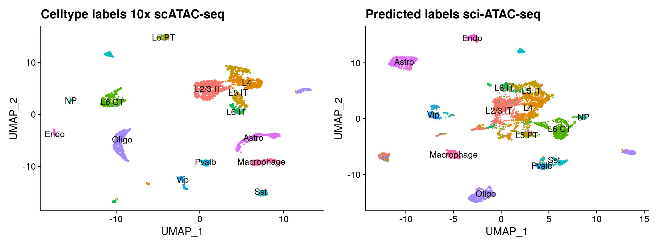
We can also use Seurat to transfer data from one dataset to another. We previously demonstrated this between scRNA-seq datasets, and between scRNA-seq and scATAC-seq datasets (https://doi.org/10.1016/j.cell.2019.05.031). Here, we demonstrate data transfer between two single-cell ATAC-seq datasets by transferring the cell type label from the 10x Genomics scATAC-seq data to the sci-ATAC-seq data.
transfer.anchors <- FindTransferAnchors(
  reference = tenx,
  query = sci,
  reference.assay = 'sciPeaks',
  query.assay = 'peaks',
  reduction = 'cca',
  features = peaks.use,
  k.filter = NA
)

predicted.id <- TransferData(
  anchorset = transfer.anchors,
  refdata = tenx$celltype,
  weight.reduction = sci[['lsi']],
  dims = 2:30
)

sci <- AddMetaData(
  object = sci,
  metadata = predicted.id
)

sci$predicted.id <- factor(sci$predicted.id, levels = levels(tenx$celltype))  # to make the colors match

p3 <- DimPlot(tenx, group.by = 'celltype', label = TRUE) + NoLegend() + ggplot2::ggtitle("Celltype labels 10x scATAC-seq")
p4 <- DimPlot(sci, group.by = 'predicted.id', label = TRUE) + NoLegend() + ggplot2::ggtitle("Predicted labels sci-ATAC-seq")
p3 + p4
Integration with Harmony
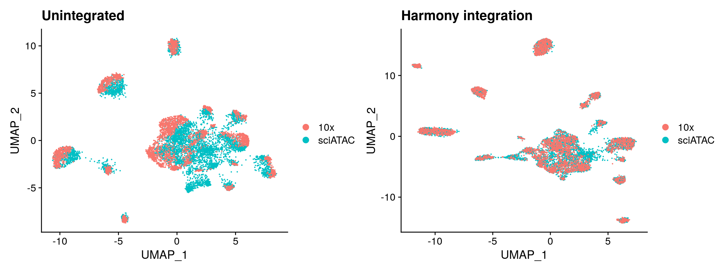
While Seurat adjusts the underlying high-dimensional data in order to correct for differences between the groups, harmony (developed by the Raychaudhuri lab) adjusts the low-dimensional cell embeddings to to reduce the dependence between cluster assignment and dataset of origin. You can read more about Harmony here.
Harmony requires a single object as input, so here we merge the sci-ATAC-seq and scATAC-seq datasets in a coordinate-aware manner using the MergeWithRegions function, and then compute LSI embeddings using the merged object. Once we have computed the LSI embeddings, we can run the RunHarmony function from the harmony package and provide the technology used as a grouping variable to remove the batch difference between the sci-ATAC-seq and 10x Genomics scATAC-seq datasets. This produces a set of “corrected” LSI embeddings that can be used for further dimension reduction with UMAP or tSNE, and for clustering.
library(harmony)

hm.integrated <- RunHarmony(
  object = unintegrated,
  group.by.vars = 'tech',
  reduction = 'lsi',
  assay.use = 'peaks',
  project.dim = FALSE
)

# re-compute the UMAP using corrected LSI embeddings
hm.integrated <- RunUMAP(hm.integrated, dims = 2:30, reduction = 'harmony')
p5 <- DimPlot(hm.integrated, group.by = 'tech', pt.size = 0.1) + ggplot2::ggtitle("Harmony integration")
p1 + p5
Session Info
## R version 4.0.1 (2020-06-06)
## Platform: x86_64-pc-linux-gnu (64-bit)
## Running under: Ubuntu 18.04.4 LTS
##
## Matrix products: default
## BLAS:   /usr/lib/x86_64-linux-gnu/blas/libblas.so.3.7.1
## LAPACK: /usr/lib/x86_64-linux-gnu/lapack/liblapack.so.3.7.1
##
## locale:
##  [1] LC_CTYPE=en_AU.UTF-8       LC_NUMERIC=C
##  [3] LC_TIME=en_US.UTF-8        LC_COLLATE=en_US.UTF-8
##  [5] LC_MONETARY=en_US.UTF-8    LC_MESSAGES=en_US.UTF-8
##  [7] LC_PAPER=en_US.UTF-8       LC_NAME=C
##  [9] LC_ADDRESS=C               LC_TELEPHONE=C
## [11] LC_MEASUREMENT=en_US.UTF-8 LC_IDENTIFICATION=C
##
## attached base packages:
## [1] stats     graphics  grDevices utils     datasets  methods   base
##
## other attached packages:
## [1] harmony_1.0       Rcpp_1.0.5        patchwork_1.0.1   Seurat_3.1.5.9009
## [5] Signac_0.2.5
##
## loaded via a namespace (and not attached):
##   [1] Rtsne_0.15                  colorspace_1.4-1
##   [3] ellipsis_0.3.1              ggridges_0.5.2
##   [5] rprojroot_1.3-2             XVector_0.28.0
##   [7] GenomicRanges_1.40.0        fs_1.4.1
##   [9] farver_2.0.3                leiden_0.3.3
##  [11] listenv_0.8.0               ggrepel_0.8.2
##  [13] ggfittext_0.9.0             codetools_0.2-16
##  [15] splines_4.0.1               knitr_1.28
##  [17] jsonlite_1.7.0              Rsamtools_2.4.0
##  [19] ica_1.0-2                   cluster_2.1.0
##  [21] png_0.1-7                   uwot_0.1.8
##  [23] sctransform_0.2.1           compiler_4.0.1
##  [25] httr_1.4.1                  backports_1.1.8
##  [27] assertthat_0.2.1            Matrix_1.2-18
##  [29] lazyeval_0.2.2              htmltools_0.5.0
##  [31] tools_4.0.1                 rsvd_1.0.3
##  [33] igraph_1.2.5                gtable_0.3.0
##  [35] glue_1.4.1                  GenomeInfoDbData_1.2.3
##  [37] RANN_2.6.1                  reshape2_1.4.4
##  [39] dplyr_1.0.0                 rappdirs_0.3.1
##  [41] Biobase_2.48.0              pkgdown_1.5.1
##  [43] vctrs_0.3.1                 Biostrings_2.56.0
##  [45] ape_5.4                     nlme_3.1-148
##  [47] rtracklayer_1.48.0          ggseqlogo_0.1
##  [49] lmtest_0.9-37               xfun_0.14
##  [51] stringr_1.4.0               globals_0.12.5
##  [53] lifecycle_0.2.0             irlba_2.3.3
##  [55] XML_3.99-0.3                future_1.17.0
##  [57] zlibbioc_1.34.0             MASS_7.3-51.6
##  [59] zoo_1.8-8                   scales_1.1.1
##  [61] parallel_4.0.1              SummarizedExperiment_1.18.1
##  [63] RColorBrewer_1.1-2          gggenes_0.4.0
##  [65] yaml_2.2.1                  memoise_1.1.0
##  [67] reticulate_1.16             pbapply_1.4-2
##  [69] gridExtra_2.3               ggplot2_3.3.2
##  [71] stringi_1.4.6               S4Vectors_0.26.1
##  [73] desc_1.2.0                  BiocGenerics_0.34.0
##  [75] BiocParallel_1.22.0         GenomeInfoDb_1.24.0
##  [77] rlang_0.4.6                 pkgconfig_2.0.3
##  [79] bitops_1.0-6                matrixStats_0.56.0
##  [81] evaluate_0.14               lattice_0.20-41
##  [83] ROCR_1.0-11                 purrr_0.3.4
##  [85] labeling_0.3                GenomicAlignments_1.24.0
##  [87] htmlwidgets_1.5.1           cowplot_1.0.0
##  [89] tidyselect_1.1.0            RcppAnnoy_0.0.16
##  [91] plyr_1.8.6                  magrittr_1.5
##  [93] R6_2.4.1                    IRanges_2.22.2
##  [95] generics_0.0.2              DelayedArray_0.14.0
##  [97] pillar_1.4.4                fitdistrplus_1.1-1
##  [99] survival_3.2-3              RCurl_1.98-1.2
## [101] tibble_3.0.1                future.apply_1.6.0
## [103] crayon_1.3.4                KernSmooth_2.23-17
## [105] plotly_4.9.2.1              rmarkdown_2.2
## [107] grid_4.0.1                  data.table_1.12.8
## [109] digest_0.6.25               tidyr_1.1.0
## [111] stats4_4.0.1                munsell_0.5.0
## [113] viridisLite_0.3.0