Visualization of genomic regions
Compiled: April 01, 2026
Source:vignettes/visualization.Rmd
visualization.RmdIn this vignette we will demonstrate how to visualize single-cell data in genome-browser-track style plots with Signac.
To demonstrate we’ll use the human PBMC dataset processed in this vignette.
There are several different genome browser style plot types available in Signac, including accessibility tracks, gene annotations, peak coordinate, genomic links, and fragment positions.
Plotting aggregated signal
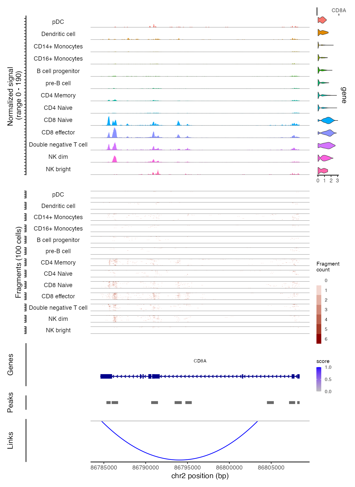
The main plotting function in Signac is CoveragePlot(),
and this computes the averaged frequency of sequenced DNA fragments for
different groups of cells within a given genomic region.
roi = "chr2-86784605-86808396"
cov_plot <- CoveragePlot(
  object = pbmc,
  region = roi,
  annotation = FALSE,
  peaks = FALSE
)
cov_plot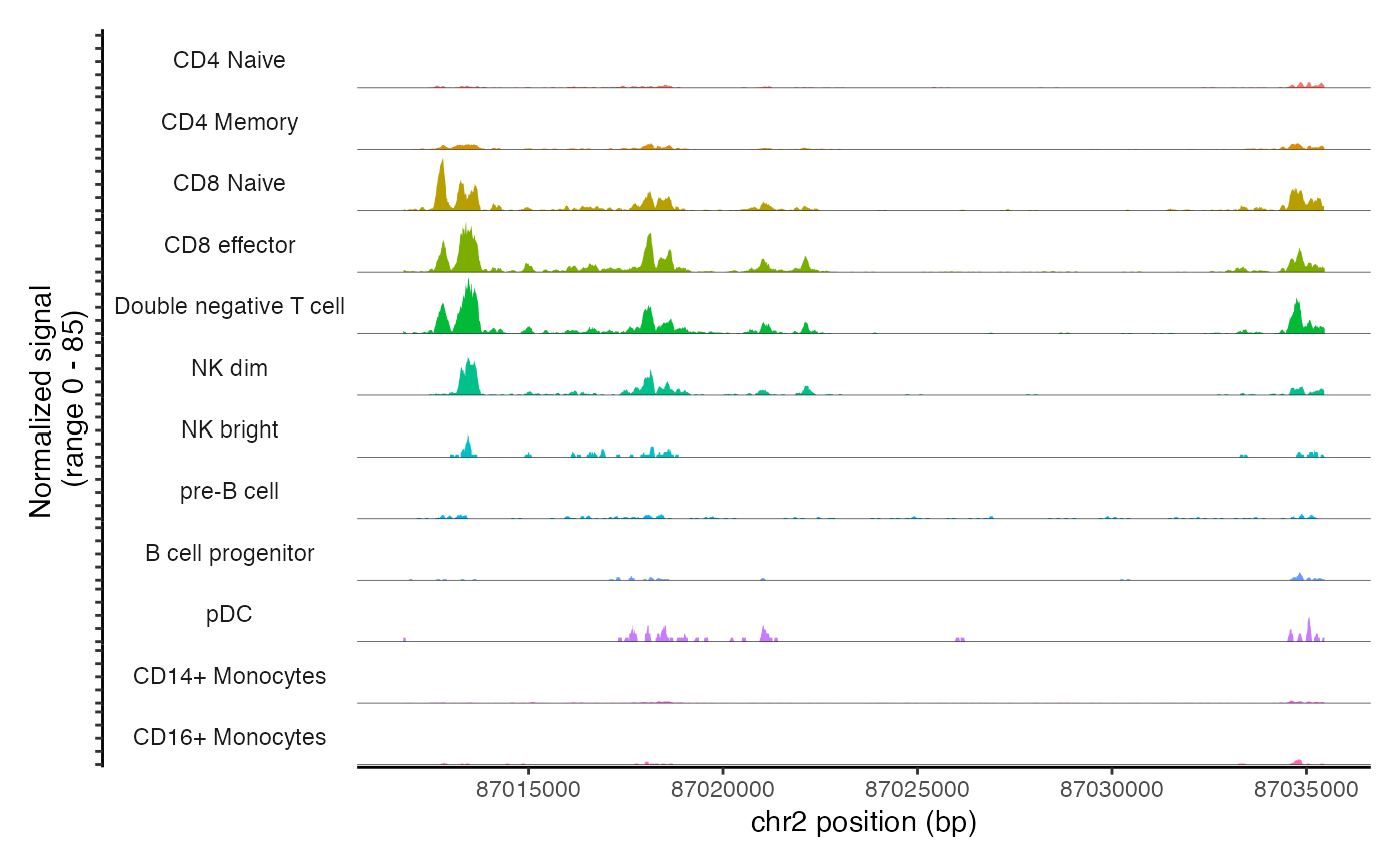
We can also request regions of the genome by gene name. This will use the gene coordinates stored in the Seurat object to determine which genomic region to plot
CoveragePlot(
  object = pbmc,
  region = "CD8A",
  annotation = FALSE,
  peaks = FALSE
)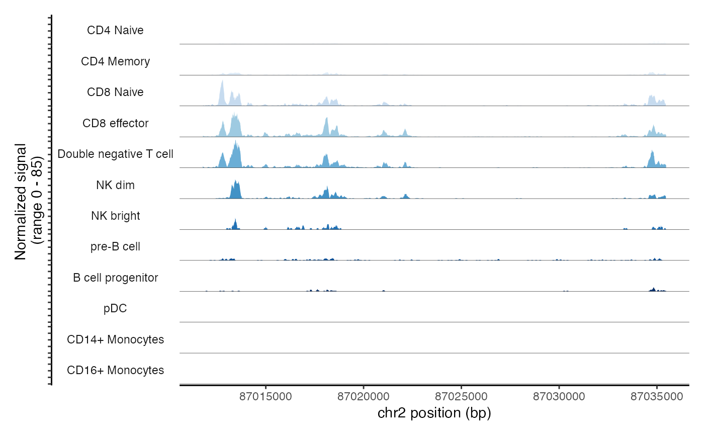
Customizing plots
All of the plots returned by Signac functions are
ggplot2 or patchwork objects, and so you can
use standard functions from ggplot2 or other packages to
further modify or customize them. For example, if we wanted to adjust
the color of the tracks generated in the plot above, we can use the
scale_fill_ functions in ggplot2, for example
scale_fill_brewer():
cov_plot + scale_fill_brewer(type = "seq", palette = 1)## Scale for fill is already present.
## Adding another scale for fill, which will replace the existing scale.## Warning in RColorBrewer::brewer.pal(n, pal): n too large, allowed maximum for palette Blues is 9
## Returning the palette you asked for with that many colors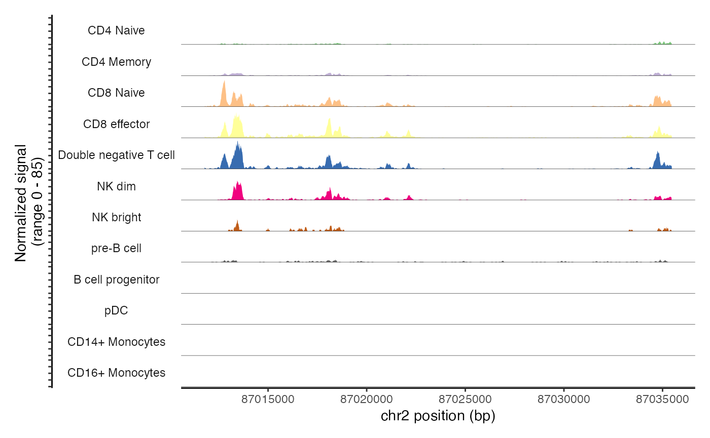
cov_plot + scale_fill_brewer(type = "qual", palette = 1)## Scale for fill is already present.
## Adding another scale for fill, which will replace the existing scale.## Warning in RColorBrewer::brewer.pal(n, pal): n too large, allowed maximum for palette Accent is 8
## Returning the palette you asked for with that many colors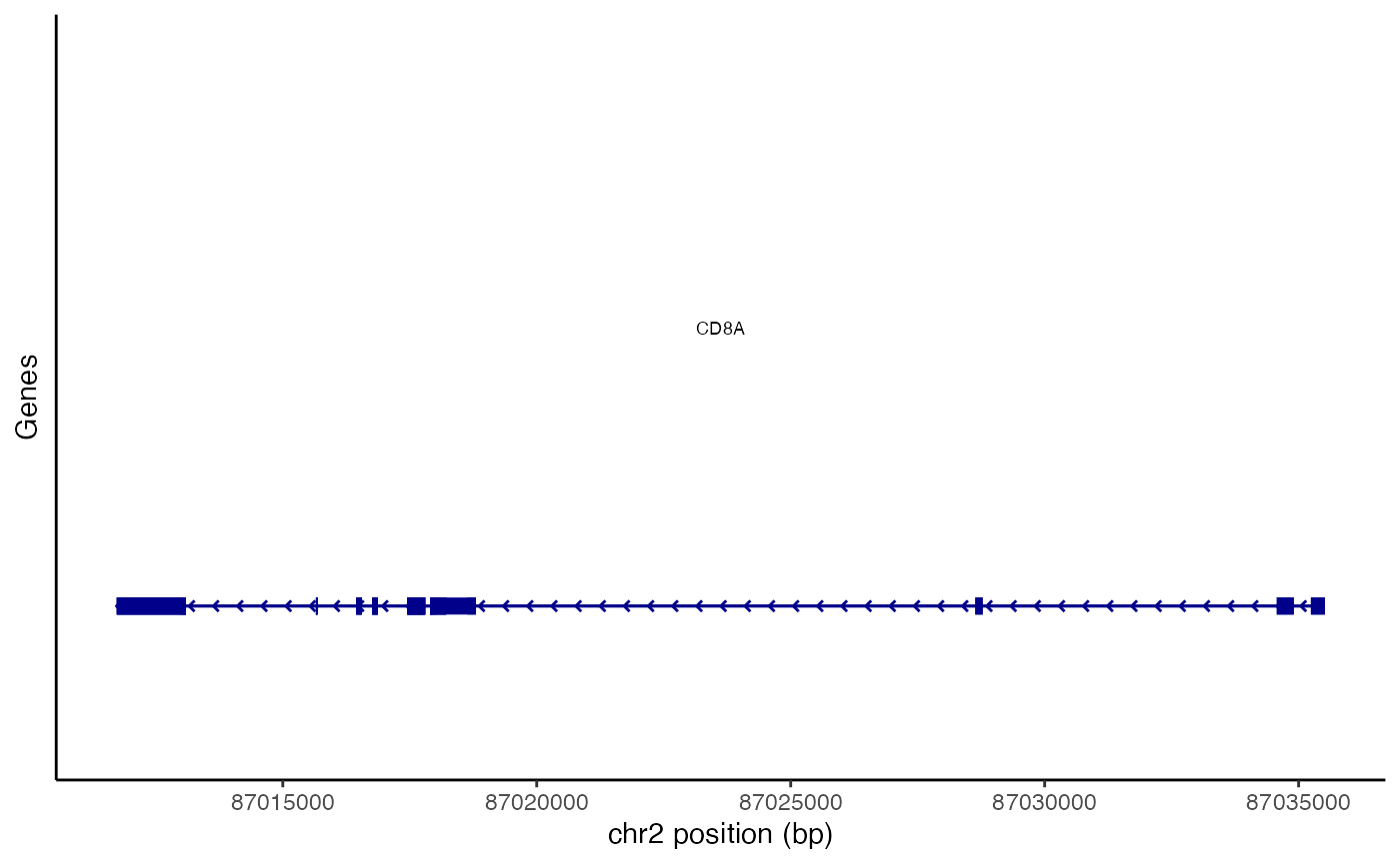
Note that for plots that are combined using Patchwork, the
& operator can be used to apply the aesthetic
adjustment to all of the plots in the object.
Plotting gene annotations
Gene annotations within a given genomic region can be plotted using
the AnnotationPlot() function.
gene_plot <- AnnotationPlot(
  object = pbmc,
  region = roi
)
gene_plot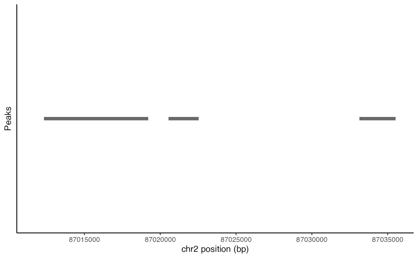
Plotting peak coordinates
Peak coordinates within a genomic region can be plotted using the
PeakPlot() function.
peak_plot <- PeakPlot(
  object = pbmc,
  region = roi
)
peak_plot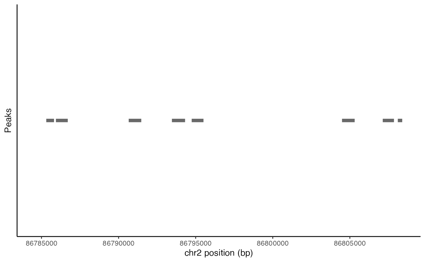
Plotting genomic links
Relationships between genomic positions can be plotted using the
LinkPlot() function. This will display an arc connecting
two linked positions, with the transparency of the arc line proportional
to a score associated with the link. These links could be used to encode
different things, including regulatory relationships (for example,
linking enhancers to the genes that they regulate), or experimental data
such as Hi-C.
Just to demonstrate how the function works, we’ve created a fake link here and added it to the PBMC dataset.
link_plot <- LinkPlot(
  object = pbmc,
  region = roi
)
link_plot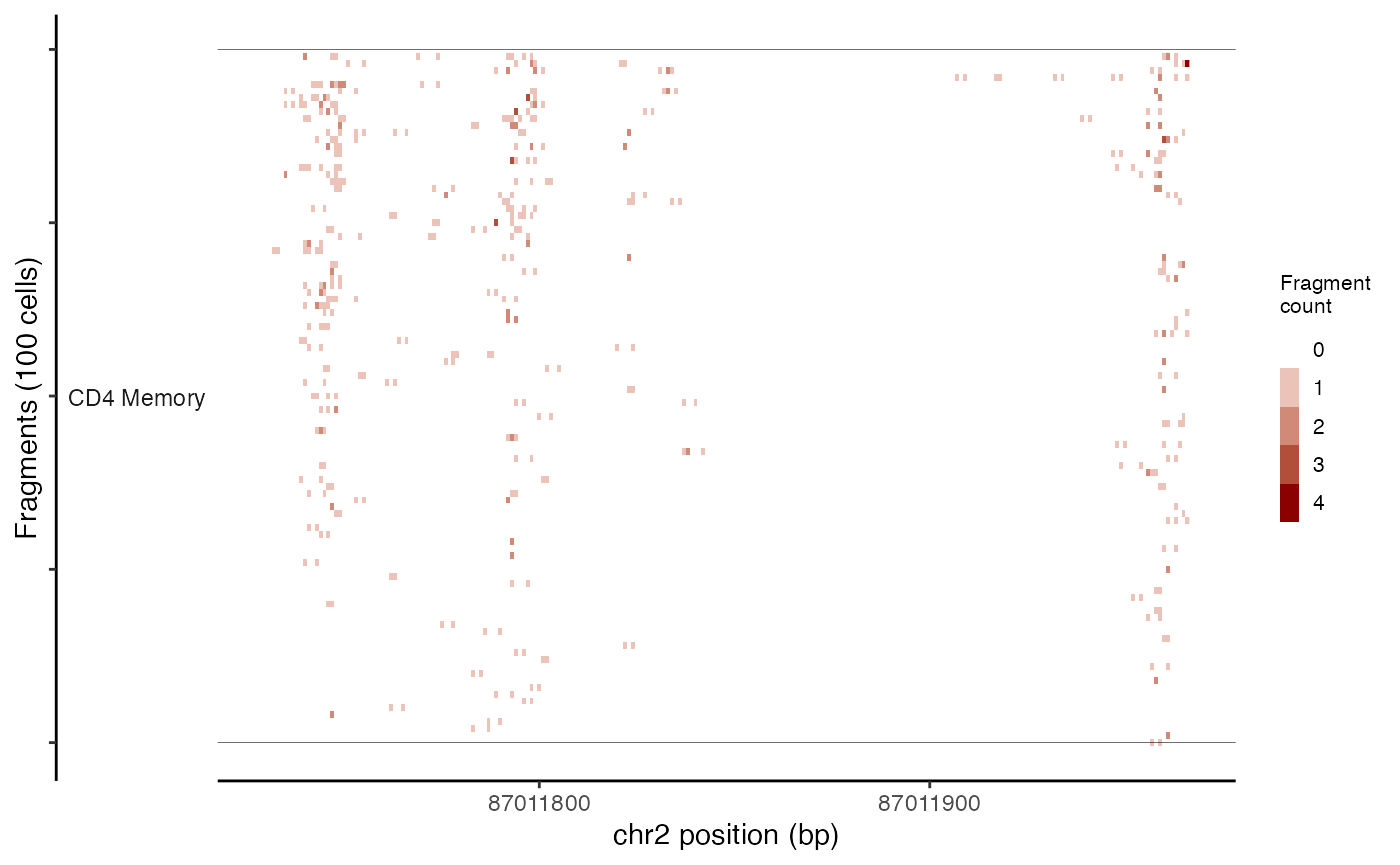
Plotting per-cell fragment abundance
While the CoveragePlot() function computes an aggregated
signal within a genomic region for different groups of cells, sometimes
it’s also useful to inspect the frequency of sequenced fragments within
a genomic region for individual cells, without aggregation.
This can be done using the TilePlot() function.
tile_plot <- TilePlot(
  object = pbmc,
  region = roi,
  idents = c("CD4 Memory", "CD8 Effector")
)
tile_plot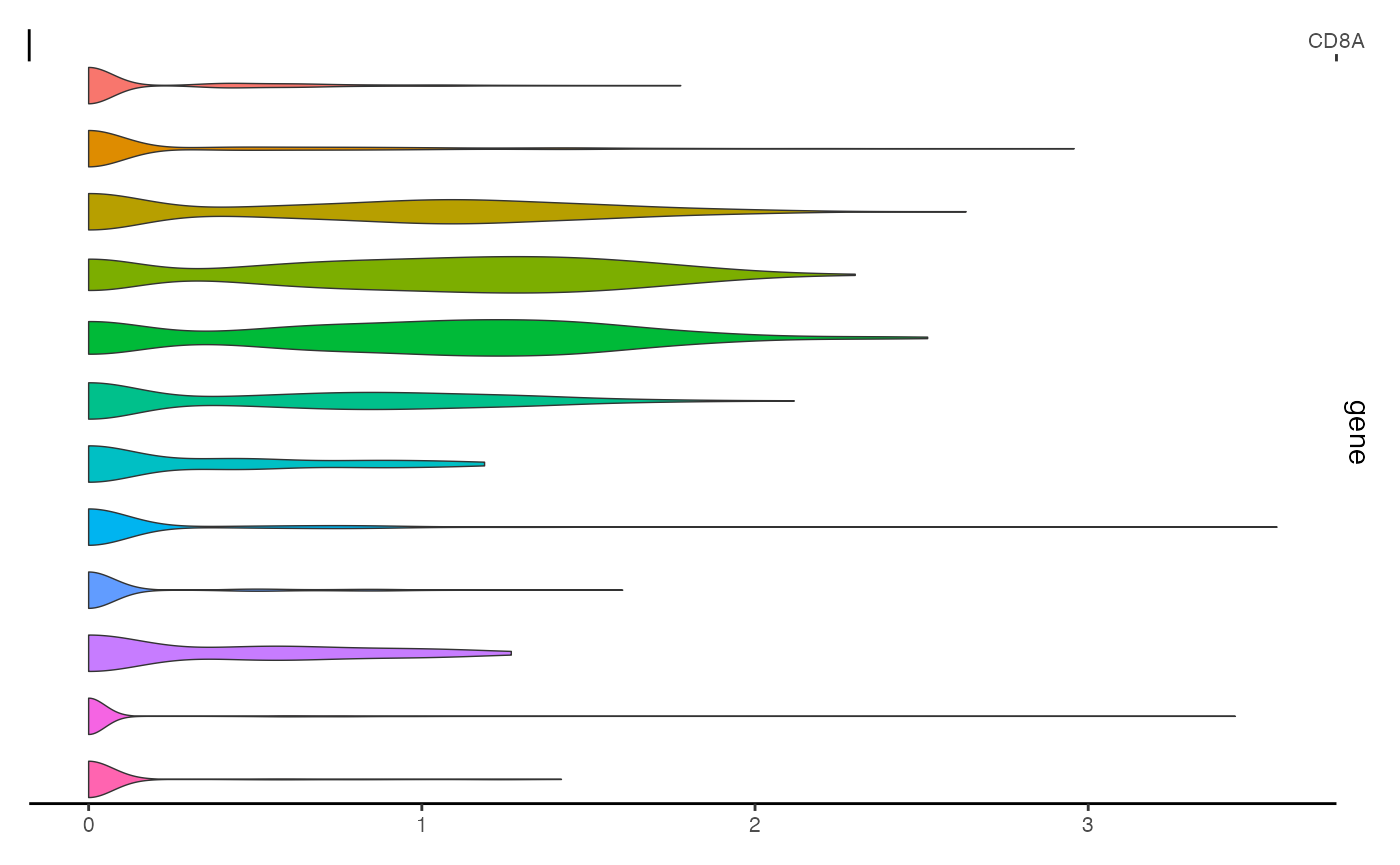
By default, this selects the top 100 cells for each group based on the total number of fragments in the genomic region. The genomic region is then tiled and the total fragments in each tile counted for each cell, and the resulting counts for each position displayed as a heatmap.
Plotting additional data alongside genomic tracks
Multimodal single-cell datasets generate multiple experimental
measurements for each cell. Several methods now exist that are capable
of measuring single-cell chromatin data (such as chromatin
accessibility) alongside other measurements from the same cell, such as
gene expression or mitochondrial genotype. In these cases it’s often
informative to visualize the multimodal data together in a single plot.
This can be achieved using the ExpressionPlot() function.
This is similar to the VlnPlot() function in Seurat, but is
designed to be incorportated with genomic track plots generated by
CoveragePlot().
expr_plot <- ExpressionPlot(
  object = pbmc,
  features = "CD8A",
  assay = "RNA"
)
expr_plot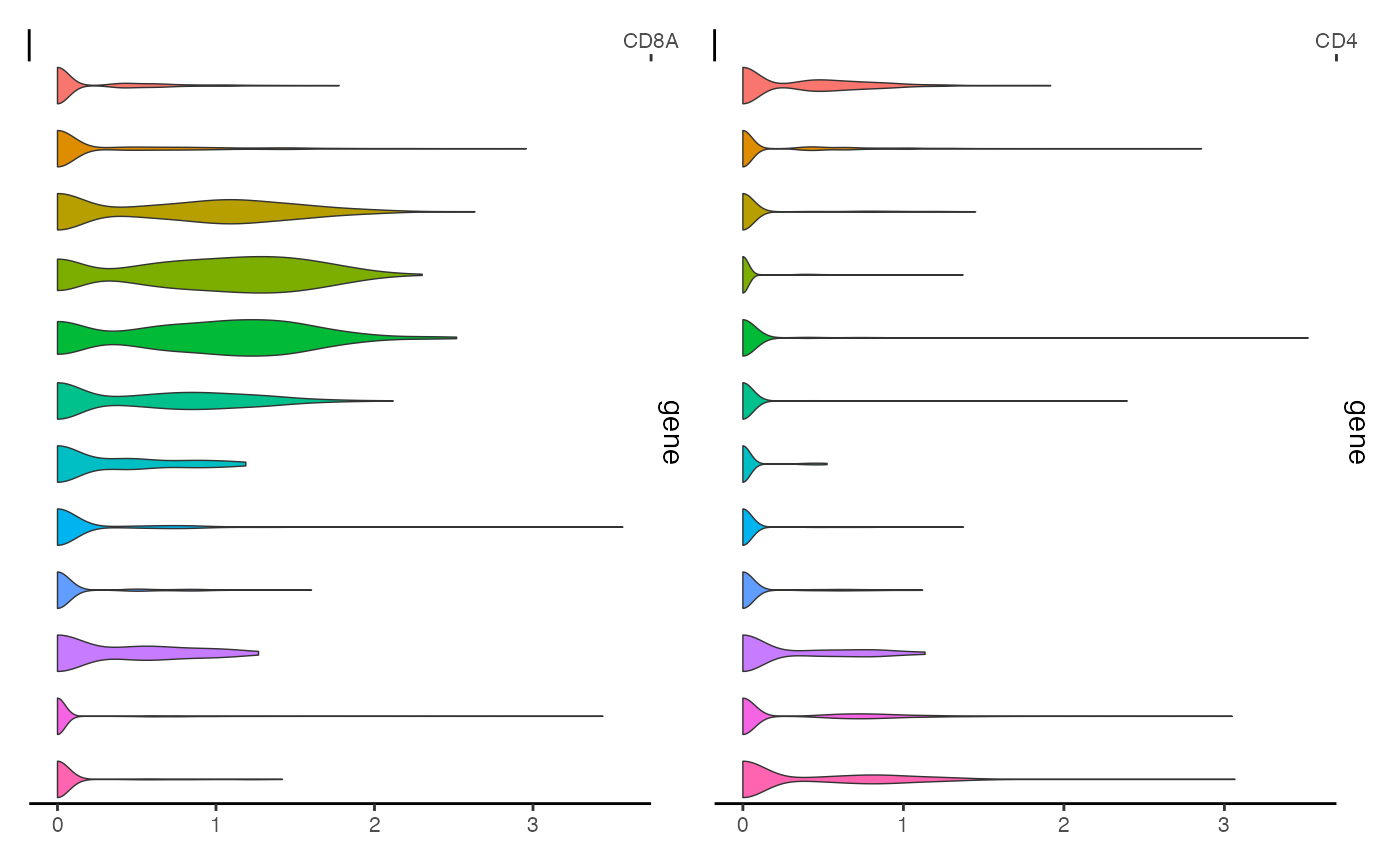
We can create similar plots for multiple genes at once simply by passing a list of gene names
ExpressionPlot(
  object = pbmc,
  features = c("CD8A", "CD4"),
  assay = "RNA"
)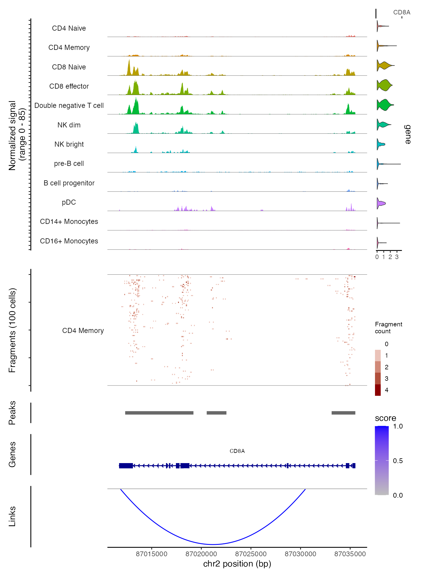
Combining genomic tracks
Above we’ve demonstrated how to generate individual tracks and panels
that can be combined into a single plot for a single genomic region.
These panels can be easily combined using the
CombineTracks() function.
CombineTracks(
  plotlist = list(cov_plot, tile_plot, peak_plot, gene_plot, link_plot),
  expression.plot = expr_plot,
  heights = c(10, 6, 1, 2, 3),
  widths = c(10, 1)
)
The heights and widths parameters control
the relative heights and widths of the individual tracks, according to
the order that the tracks appear in the plotlist. The
CombineTracks() function ensures that the tracks are
aligned vertically and horizontally, and moves the x-axis labels
(describing the genomic position) to the bottom of the combined
tracks.
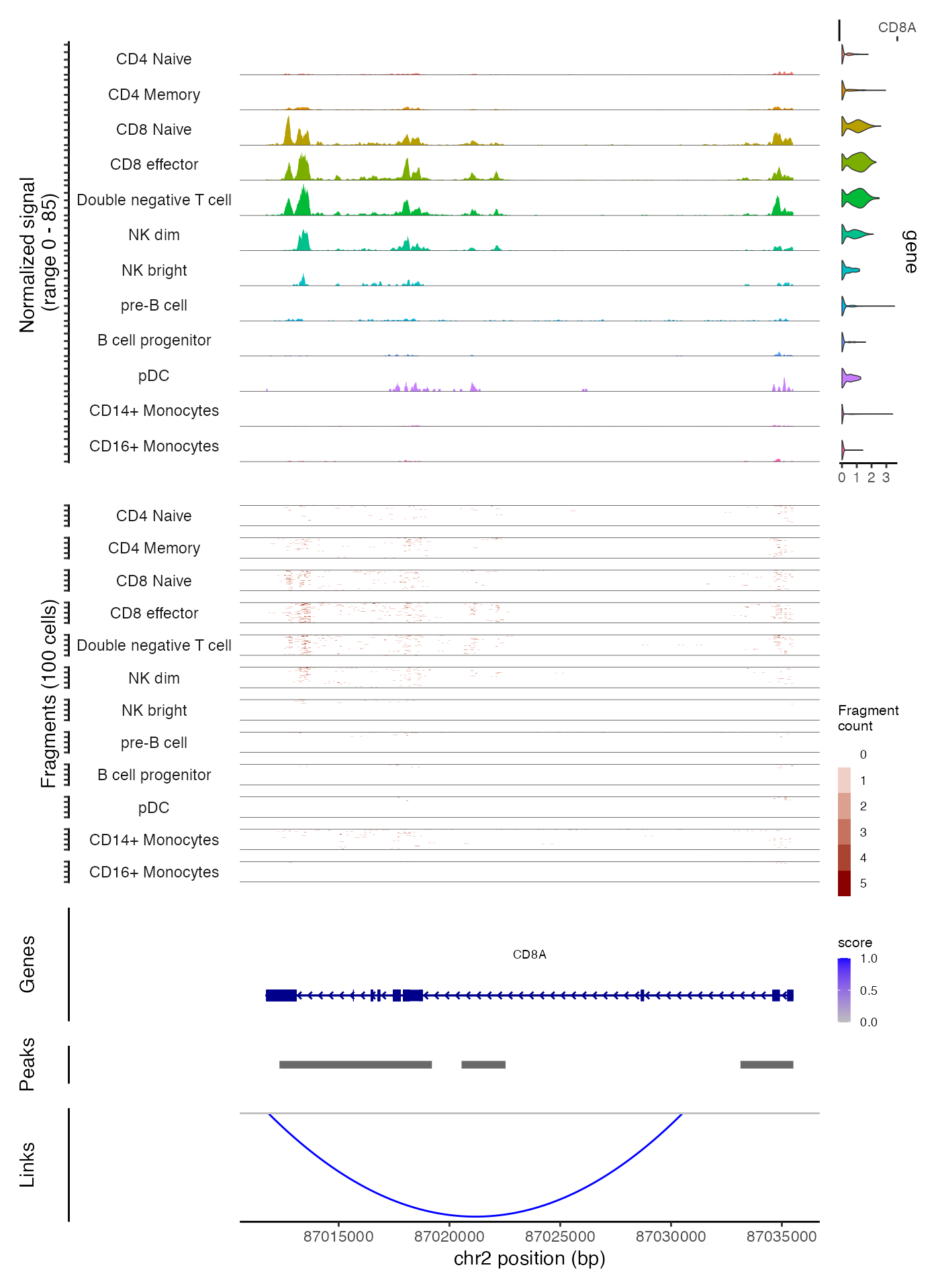
Generating multiple tracks
Above we’ve shown how to create genomic plot panels individually and
how to combine them. This allows more control over how each panel is
constructed and how they’re combined, but involves multiple steps. For
convenience, we’ve included the ability to generate and combine
different panels automatically in the CoveragePlot()
function, through the annotation, peaks,
tile, and features arguments. We can generate
a similar plot to that shown above in a single function call:
CoveragePlot(
  object = pbmc,
  region = roi,
  features = "CD8A",
  annotation = TRUE,
  peaks = TRUE,
  tile = TRUE,
  links = TRUE
)
Notice that in this example we create the tile plot for every group of cells that is shown in the coverage track, whereas above we were able to create a plot that showed the aggregated coverage for all groups of cells and the tile plot for only the CD4 memory cells and the CD8 effector cells. A higher degree of customization is possible when creating each track separately.
Interactive visualization
Above we demonstrated the different types of plots that can be
constructed using Signac. Often when exploring genomic data it’s useful
to be able to interactively browse through different regions of the
genome and adjust tracks on the fly. This can be done in Signac using
the CoverageBrowser() function. This provides all the same
functionality of the CoveragePlot() function, except that
we can scroll upstream/downstream, zoom in/out of regions, navigate to
new region, and adjust which tracks are shown or how the cells are
grouped. In exploring the data interactively, often you will find
interesting plots that you’d like to save for viewing later. We’ve
included a “Save plot” button that will add the current plot to a list
of plots that is returned when the interactive session is ended. Here’s
a recorded demonstration of the CoverageBrowser()
function:
Session Info
## R version 4.5.1 (2025-06-13)
## Platform: aarch64-apple-darwin20
## Running under: macOS Tahoe 26.4
##
## Matrix products: default
## BLAS:   /Library/Frameworks/R.framework/Versions/4.5-arm64/Resources/lib/libRblas.0.dylib
## LAPACK: /Library/Frameworks/R.framework/Versions/4.5-arm64/Resources/lib/libRlapack.dylib;  LAPACK version 3.12.1
##
## locale:
## [1] en_US.UTF-8/en_US.UTF-8/en_US.UTF-8/C/en_US.UTF-8/en_US.UTF-8
##
## time zone: Asia/Singapore
## tzcode source: internal
##
## attached base packages:
## [1] stats4    stats     graphics  grDevices utils     datasets  methods
## [8] base
##
## other attached packages:
## [1] GenomicRanges_1.62.1 Seqinfo_1.0.0        IRanges_2.44.0
## [4] S4Vectors_0.48.0     BiocGenerics_0.56.0  generics_0.1.4
## [7] ggplot2_4.0.2        Signac_1.17.0
##
## loaded via a namespace (and not attached):
##  [1] tidyselect_1.2.1         dplyr_1.2.0              farver_2.1.2
##  [4] Biostrings_2.78.0        S7_0.2.1                 bitops_1.0-9
##  [7] fastmap_1.2.0            tweenr_2.0.3             stringfish_0.18.0
## [10] digest_0.6.39            dotCall64_1.2            lifecycle_1.0.5
## [13] SeuratObject_5.3.0.9002  magrittr_2.0.4           compiler_4.5.1
## [16] rlang_1.1.7              sass_0.4.10              tools_4.5.1
## [19] yaml_2.3.12              data.table_1.18.2.1      knitr_1.51
## [22] labeling_0.4.3           htmlwidgets_1.6.4        sp_2.2-1
## [25] RColorBrewer_1.1-3       BiocParallel_1.44.0      withr_3.0.2
## [28] purrr_1.2.1              desc_1.4.3               polyclip_1.10-7
## [31] grid_4.5.1               future_1.70.0            progressr_0.18.0
## [34] MASS_7.3-65              globals_0.19.1           scales_1.4.0
## [37] dichromat_2.0-0.1        cli_3.6.5                rmarkdown_2.31
## [40] crayon_1.5.3             ragg_1.5.0               otel_0.2.0
## [43] RcppParallel_5.1.11-1    future.apply_1.20.2      RSpectra_0.16-2
## [46] httr_1.4.8               RcppRoll_0.3.2           ggforce_0.5.0
## [49] pbapply_1.7-4            cachem_1.1.0             parallel_4.5.1
## [52] XVector_0.50.0           matrixStats_1.5.0        vctrs_0.7.2
## [55] Matrix_1.7-4             jsonlite_2.0.0           patchwork_1.3.2
## [58] listenv_0.10.1           systemfonts_1.3.1        jquerylib_0.1.4
## [61] tidyr_1.3.2              glue_1.8.0               parallelly_1.46.1
## [64] spam_2.11-3              pkgdown_2.2.0            codetools_0.2-20
## [67] stringi_1.8.7            gtable_0.3.6             GenomeInfoDb_1.46.2
## [70] UCSC.utils_1.6.1         tibble_3.3.1             pillar_1.11.1
## [73] htmltools_0.5.9          R6_2.6.1                 textshaping_1.0.4
## [76] sparseMatrixStats_1.22.0 evaluate_1.0.5           lattice_0.22-9
## [79] Rsamtools_2.26.0         bslib_0.10.0             Rcpp_1.1.1
## [82] fastmatch_1.1-8          qs2_0.1.7                xfun_0.57
## [85] fs_2.0.1                 MatrixGenerics_1.22.0    pkgconfig_2.0.3