Building trajectories with Monocle 3
Compiled: April 01, 2026
Source:vignettes/monocle.Rmd
monocle.RmdIn this vignette we will demonstrate how to construct cell trajectories with Monocle 3 using single-cell ATAC-seq data. Please see the Monocle 3 website for information about installing Monocle 3.
To facilitate conversion between the Seurat (used by Signac) and CellDataSet (used by Monocle 3) formats, we will use a conversion function in the SeuratWrappers package available on GitHub.
Data loading
We will use a single-cell ATAC-seq dataset containing human CD34+ hematopoietic stem and progenitor cells published by Satpathy and Granja et al. (2019, Nature Biotechnology).
The processed dataset is available on NCBI GEO here: https://www.ncbi.nlm.nih.gov/geo/query/acc.cgi?acc=GSE129785
Note that the fragment file is present inside the
GSE129785_RAW.tar archive, and the index for the fragment
file is not supplied. You can index the file yourself using tabix, for example:
tabix -p bed <fragment_file>.
First we will load the dataset and perform some standard preprocessing using Signac.
library(Signac)
library(Seurat)
library(SeuratWrappers)
library(monocle3)
library(Matrix)
library(ggplot2)
library(patchwork)
filepath <- "GSE129785_scATAC-Hematopoiesis-CD34"

peaks <- read.table(paste0(filepath, ".peaks.txt.gz"), header = TRUE)
cells <- read.table(paste0(filepath, ".cell_barcodes.txt.gz"), header = TRUE, stringsAsFactors = FALSE)
rownames(cells) <- make.unique(cells$Barcodes)

mtx <- readMM(file = paste0(filepath, ".mtx"))
mtx <- as(object = mtx, Class = "CsparseMatrix")
colnames(mtx) <- rownames(cells)
rownames(mtx) <- peaks$Feature
bone_assay <- CreateChromatinAssay(
  counts = mtx,
  min.cells = 5,
  fragments = "GSM3722029_CD34_Progenitors_Rep1_fragments.tsv.gz",
  sep = c("_", "_"),
  genome = "hg19"
)
bone <- CreateSeuratObject(
  counts = bone_assay,
  meta.data = cells,
  assay = "ATAC"
)

# The dataset contains multiple cell types
# We can subset to include just one replicate of CD34+ progenitor cells
bone <- bone[, bone$Group_Barcode == "CD34_Progenitors_Rep1"]

# add cell type annotations from the original paper
cluster_names <- c("HSC",   "MEP",  "CMP-BMP",  "LMPP", "CLP",  "Pro-B",    "Pre-B",    "GMP",
                  "MDP",    "pDC",  "cDC",  "Monocyte-1",   "Monocyte-2",   "Naive-B",  "Memory-B",
                  "Plasma-cell",    "Basophil", "Immature-NK",  "Mature-NK1",   "Mature-NK2",   "Naive-CD4-T1",
                  "Naive-CD4-T2",   "Naive-Treg",   "Memory-CD4-T", "Treg", "Naive-CD8-T1", "Naive-CD8-T2",
                  "Naive-CD8-T3",   "Central-memory-CD8-T", "Effector-memory-CD8-T",    "Gamma delta T")
num.labels <- length(cluster_names)
names(cluster_names) <- paste0( rep("Cluster", num.labels), seq(num.labels) )
new.md <- cluster_names[as.character(bone$Clusters)]
names(new.md) <- Cells(bone)
bone$celltype <- new.md

bone[["ATAC"]]
## ChromatinAssay data with 570650 features for 9913 cells
## Variable features: 0
## Genome: hg19
## Annotation present: FALSE
## Motifs present: FALSE
## Fragment files: 1Next we can add gene annotations for the hg19 genome to the object. This will be useful for computing quality control metrics (TSS enrichment score) and plotting.
library(EnsDb.Hsapiens.v75)

# extract gene annotations from EnsDb
annotations <- GetGRangesFromEnsDb(ensdb = EnsDb.Hsapiens.v75)

# change to UCSC style since the data was mapped to hg19
seqlevels(annotations) <- paste0('chr', seqlevels(annotations))
genome(annotations) <- "hg19"

# add the gene information to the object
Annotation(bone) <- annotations
Quality control
We’ll compute TSS enrichment, nucleosome signal score, and the percentage of counts in genomic blacklist regions for each cell, and use these metrics to help remove low quality cells from the datasets.
bone <- TSSEnrichment(bone)
bone <- NucleosomeSignal(bone)

# blacklist regions for hg19
library(AnnotationHub)
ah <- AnnotationHub()
blacklist_hg19 <- ah[['AH107314']]

bone$blacklist_fraction <- FractionCountsInRegion(bone, regions = blacklist_hg19)
VlnPlot(
  object = bone,
  features = c("nCount_ATAC", "TSS.enrichment", "nucleosome_signal", "blacklist_fraction"),
  pt.size = 0.1,
  ncol = 4
)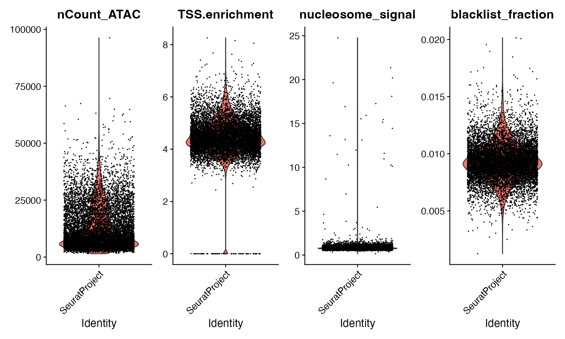
bone <- bone[, (bone$nCount_ATAC < 50000) &
               (bone$TSS.enrichment > 2) &
               (bone$nucleosome_signal < 5)]
Dataset preprocessing
Next we can run a standard scATAC-seq analysis pipeline using Signac to perform dimension reduction, clustering, and cell type annotation.
bone <- FindTopFeatures(bone, min.cells = 10)
bone <- RunTFIDF(bone)
bone <- RunSVD(bone, n = 100)
DepthCor(bone)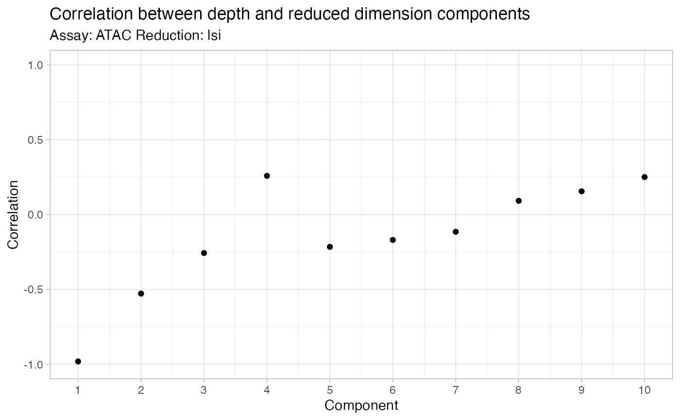
bone <- RunUMAP(
  bone,
  reduction = "lsi",
  dims = 2:50,
  reduction.name = "UMAP"
)
bone <- FindNeighbors(bone, dims = 2:50, reduction = "lsi")
bone <- FindClusters(bone, resolution = 0.8, algorithm = 3)
## Modularity Optimizer version 1.3.0 by Ludo Waltman and Nees Jan van Eck
##
## Number of nodes: 9765
## Number of edges: 433497
##
## Running smart local moving algorithm...
## Maximum modularity in 10 random starts: 0.8475
## Number of communities: 18
## Elapsed time: 4 seconds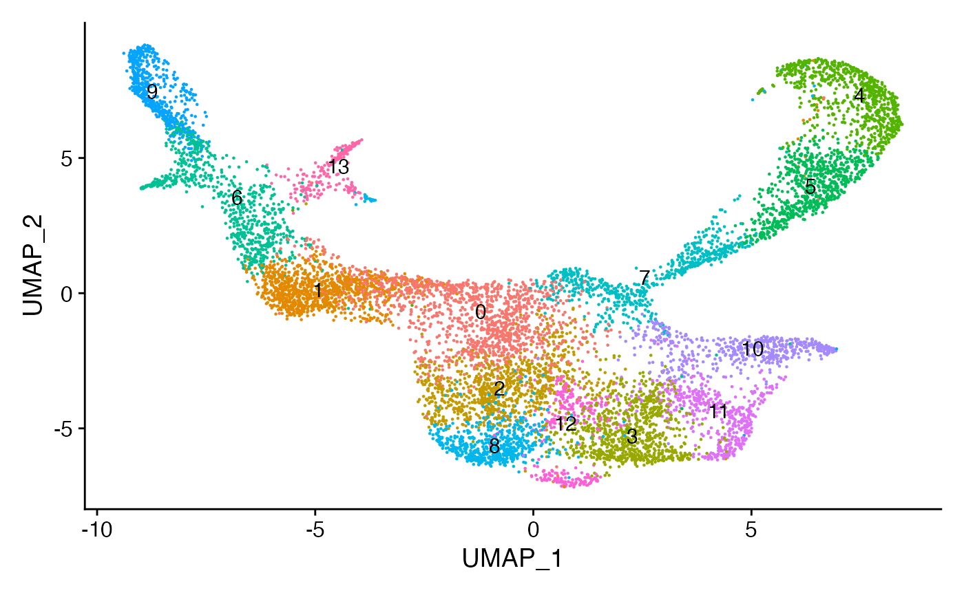
Assign each cluster to the most common cell type based on the original annotations from the paper.
for(i in levels(bone)) {
  cells_to_reid <- WhichCells(bone, idents = i)
  newid <- names(sort(table(bone$celltype[cells_to_reid]),decreasing=TRUE))[1]
  Idents(bone, cells = cells_to_reid) <- newid
}
bone$assigned_celltype <- Idents(bone)
DimPlot(bone, label = TRUE)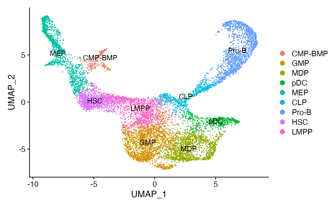
Next we can subset the different lineages and create a trajectory for each lineage. Another way to build the trajectories is to use the whole dataset and build separate pseudotime trajectories for the different cell partitions found by Monocle 3.
DefaultAssay(bone) <- "ATAC"

erythroid <- bone[,  bone$assigned_celltype %in% c("HSC", "MEP", "CMP-BMP")]
lymphoid <- bone[, bone$assigned_celltype %in% c("HSC", "LMPP", "GMP", "CLP", "Pro-B", "pDC", "MDP", "GMP")]
Building trajectories with Monocle 3
We can convert the Seurat object to a CellDataSet object using the
as.cell_data_set() function from SeuratWrappers
and build the trajectories using Monocle 3. We’ll do this separately for
erythroid and lymphoid lineages, but you could explore other strategies
building a trajectory for all lineages together.
erythroid.cds <- as.cell_data_set(erythroid)
erythroid.cds <- cluster_cells(cds = erythroid.cds, reduction_method = "UMAP")
erythroid.cds <- learn_graph(erythroid.cds, use_partition = TRUE)

lymphoid.cds <- as.cell_data_set(lymphoid)
lymphoid.cds <- cluster_cells(cds = lymphoid.cds, reduction_method = "UMAP")
lymphoid.cds <- learn_graph(lymphoid.cds, use_partition = TRUE)
To compute pseudotime estimates for each trajectory we need to decide
what the start of each trajectory is. In our case, we know that the
hematopoietic stem cells are the progenitors of other cell types in the
trajectory, so we can set these cells as the root of the trajectory.
Monocle 3 includes an interactive function to select cells as the root
nodes in the graph. This function will be launched if calling
order_cells() without specifying the
root_cells parameter. Here we’ve pre-selected some cells as
the root, and saved these to a file for reproducibility. This file can
be downloaded here.
# load the pre-selected HSCs
hsc <- readLines("../hsc_cells.txt")
# order cells
erythroid.cds <- order_cells(erythroid.cds, reduction_method = "UMAP", root_cells = hsc)
lymphoid.cds <- order_cells(lymphoid.cds, reduction_method = "UMAP", root_cells = hsc)
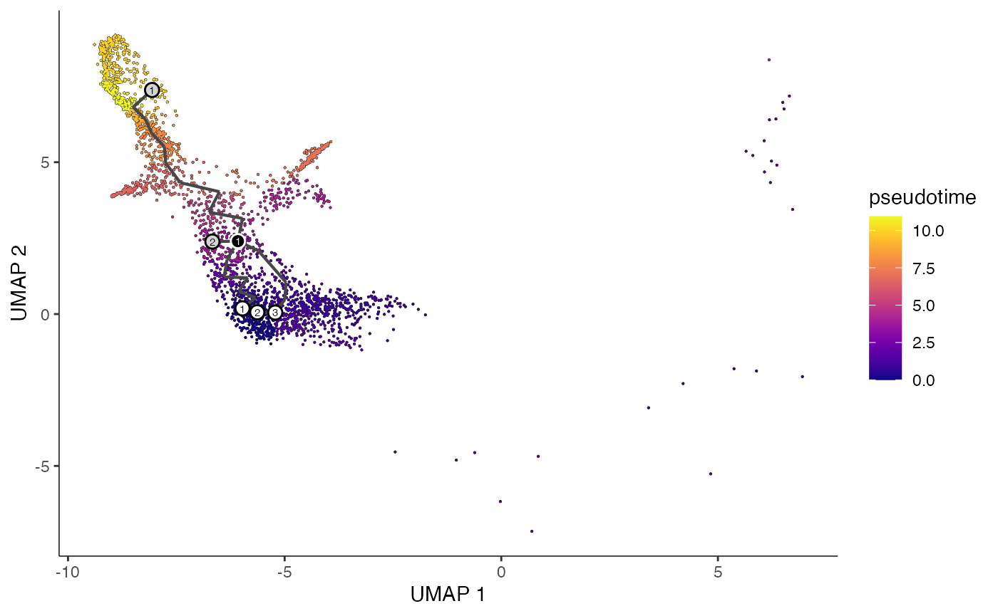
# plot trajectories colored by pseudotime
plot_cells(
cds = erythroid.cds,
color_cells_by = "pseudotime",
show_trajectory_graph = TRUE
)
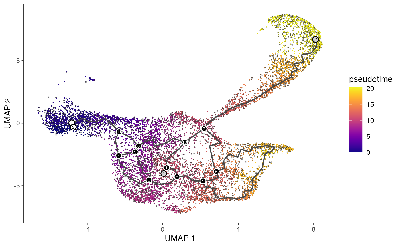
plot_cells(
  cds = lymphoid.cds,
  color_cells_by = "pseudotime",
  show_trajectory_graph = TRUE
)
Extract the pseudotime values and add to the Seurat object
bone <- AddMetaData(
  object = bone,
  metadata = erythroid.cds@principal_graph_aux@listData$UMAP$pseudotime,
  col.name = "Erythroid"
)

bone <- AddMetaData(
  object = bone,
  metadata = lymphoid.cds@principal_graph_aux@listData$UMAP$pseudotime,
  col.name = "Lymphoid"
)
FeaturePlot(bone, c("Erythroid", "Lymphoid"), pt.size = 0.1) & scale_color_viridis_c()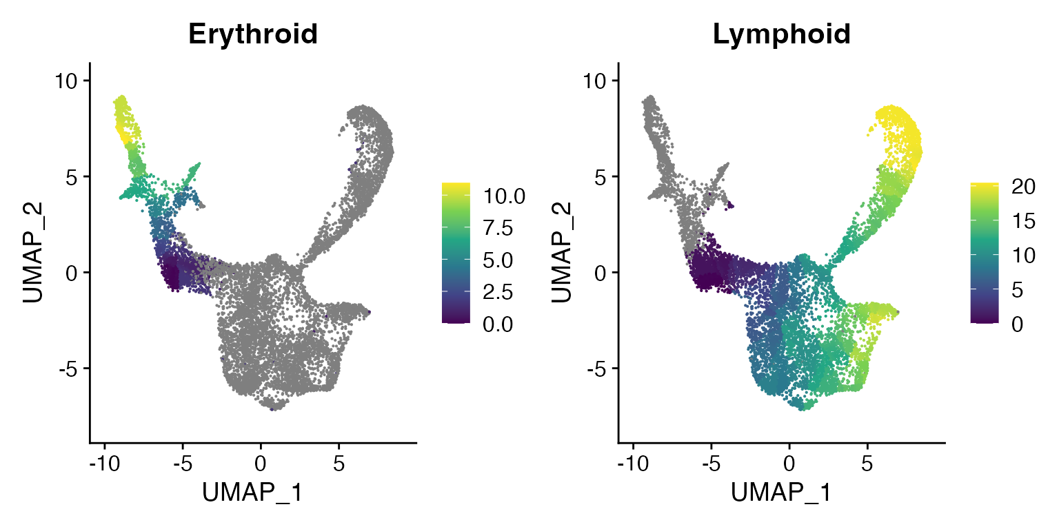
Acknowledgements
Thanks to the developers of Monocle 3, especially Cole Trapnell, Hannah Pliner, and members of the Trapnell lab. If you use Monocle please cite the Monocle papers.
Session Info
## R version 4.5.1 (2025-06-13)
## Platform: aarch64-apple-darwin20
## Running under: macOS Tahoe 26.4
##
## Matrix products: default
## BLAS:   /Library/Frameworks/R.framework/Versions/4.5-arm64/Resources/lib/libRblas.0.dylib
## LAPACK: /Library/Frameworks/R.framework/Versions/4.5-arm64/Resources/lib/libRlapack.dylib;  LAPACK version 3.12.1
##
## locale:
## [1] en_US.UTF-8/en_US.UTF-8/en_US.UTF-8/C/en_US.UTF-8/en_US.UTF-8
##
## time zone: Asia/Singapore
## tzcode source: internal
##
## attached base packages:
## [1] stats4    stats     graphics  grDevices utils     datasets  methods
## [8] base
##
## other attached packages:
##  [1] future_1.70.0               AnnotationHub_4.0.0
##  [3] BiocFileCache_3.0.0         dbplyr_2.5.2
##  [5] EnsDb.Hsapiens.v75_2.99.0   ensembldb_2.34.0
##  [7] AnnotationFilter_1.34.0     GenomicFeatures_1.62.0
##  [9] AnnotationDbi_1.72.0        patchwork_1.3.2
## [11] ggplot2_4.0.2               Matrix_1.7-4
## [13] monocle3_1.4.26             SingleCellExperiment_1.32.0
## [15] SummarizedExperiment_1.40.0 GenomicRanges_1.62.1
## [17] Seqinfo_1.0.0               IRanges_2.44.0
## [19] S4Vectors_0.48.0            MatrixGenerics_1.22.0
## [21] matrixStats_1.5.0           Biobase_2.70.0
## [23] BiocGenerics_0.56.0         generics_0.1.4
## [25] SeuratWrappers_0.4.0        Seurat_5.4.0
## [27] SeuratObject_5.3.0.9002     sp_2.2-1
## [29] Signac_1.17.0
##
## loaded via a namespace (and not attached):
##   [1] fs_2.0.1                 ProtGenerics_1.42.0      spatstat.sparse_3.1-0
##   [4] bitops_1.0-9             httr_1.4.8               RColorBrewer_1.1-3
##   [7] backports_1.5.0          tools_4.5.1              sctransform_0.4.3
##  [10] R6_2.6.1                 lazyeval_0.2.2           uwot_0.2.4
##  [13] withr_3.0.2              gridExtra_2.3            progressr_0.18.0
##  [16] cli_3.6.5                textshaping_1.0.4        spatstat.explore_3.7-0
##  [19] fastDummies_1.7.5        labeling_0.4.3           sass_0.4.10
##  [22] S7_0.2.1                 spatstat.data_3.1-9      proxy_0.4-29
##  [25] ggridges_0.5.7           pbapply_1.7-4            pkgdown_2.2.0
##  [28] Rsamtools_2.26.0         systemfonts_1.3.1        foreign_0.8-91
##  [31] R.utils_2.13.0           dichromat_2.0-0.1        parallelly_1.46.1
##  [34] BSgenome_1.78.0          rstudioapi_0.18.0        RSQLite_2.4.6
##  [37] BiocIO_1.20.0            ica_1.0-3                spatstat.random_3.4-4
##  [40] dplyr_1.2.0              ggbeeswarm_0.7.3         abind_1.4-8
##  [43] R.methodsS3_1.8.2        lifecycle_1.0.5          yaml_2.3.12
##  [46] SparseArray_1.10.8       Rtsne_0.17               grid_4.5.1
##  [49] blob_1.3.0               promises_1.5.0           crayon_1.5.3
##  [52] miniUI_0.1.2             lattice_0.22-9           cowplot_1.2.0
##  [55] cigarillo_1.0.0          KEGGREST_1.50.0          pillar_1.11.1
##  [58] knitr_1.51               rjson_0.2.23             boot_1.3-32
##  [61] future.apply_1.20.2      codetools_0.2-20         fastmatch_1.1-8
##  [64] glue_1.8.0               leidenbase_0.1.36        spatstat.univar_3.1-6
##  [67] data.table_1.18.2.1      remotes_2.5.0            vctrs_0.7.2
##  [70] png_0.1-9                spam_2.11-3              Rdpack_2.6.6
##  [73] gtable_0.3.6             assertthat_0.2.1         cachem_1.1.0
##  [76] xfun_0.57                rbibutils_2.4.1          S4Arrays_1.10.1
##  [79] mime_0.13                reformulas_0.4.4         survival_3.8-6
##  [82] RcppRoll_0.3.2           fitdistrplus_1.2-6       ROCR_1.0-12
##  [85] nlme_3.1-168             bit64_4.6.0-1            filelock_1.0.3
##  [88] RcppAnnoy_0.0.23         GenomeInfoDb_1.46.2      bslib_0.10.0
##  [91] irlba_2.3.7              vipor_0.4.7              rpart_4.1.24
##  [94] KernSmooth_2.23-26       otel_0.2.0               colorspace_2.1-2
##  [97] DBI_1.3.0                Hmisc_5.2-5              nnet_7.3-20
## [100] ggrastr_1.0.2            tidyselect_1.2.1         bit_4.6.0
## [103] compiler_4.5.1           curl_7.0.0               httr2_1.2.2
## [106] htmlTable_2.4.3          desc_1.4.3               DelayedArray_0.36.0
## [109] plotly_4.12.0            stringfish_0.18.0        rtracklayer_1.70.1
## [112] checkmate_2.3.4          scales_1.4.0             lmtest_0.9-40
## [115] rappdirs_0.3.4           stringr_1.6.0            digest_0.6.39
## [118] goftest_1.2-3            spatstat.utils_3.2-1     minqa_1.2.8
## [121] rmarkdown_2.31           XVector_0.50.0           htmltools_0.5.9
## [124] pkgconfig_2.0.3          base64enc_0.1-6          lme4_1.1-38
## [127] sparseMatrixStats_1.22.0 fastmap_1.2.0            rlang_1.1.7
## [130] htmlwidgets_1.6.4        UCSC.utils_1.6.1         shiny_1.13.0
## [133] farver_2.1.2             jquerylib_0.1.4          zoo_1.8-15
## [136] jsonlite_2.0.0           BiocParallel_1.44.0      R.oo_1.27.1
## [139] VariantAnnotation_1.56.0 RCurl_1.98-1.18          magrittr_2.0.4
## [142] Formula_1.2-5            dotCall64_1.2            Rcpp_1.1.1
## [145] viridis_0.6.5            reticulate_1.45.0        stringi_1.8.7
## [148] MASS_7.3-65              plyr_1.8.9               parallel_4.5.1
## [151] listenv_0.10.1           ggrepel_0.9.7            deldir_2.0-4
## [154] Biostrings_2.78.0        splines_4.5.1            tensor_1.5.1
## [157] igraph_2.2.2             spatstat.geom_3.7-0      RcppHNSW_0.6.0
## [160] qs2_0.1.7                reshape2_1.4.5           BiocVersion_3.22.0
## [163] XML_3.99-0.23            evaluate_1.0.5           biovizBase_1.58.0
## [166] RcppParallel_5.1.11-1    BiocManager_1.30.27      nloptr_2.2.1
## [169] httpuv_1.6.16            RANN_2.6.2               tidyr_1.3.2
## [172] purrr_1.2.1              polyclip_1.10-7          scattermore_1.2
## [175] rsvd_1.0.5               xtable_1.8-8             restfulr_0.0.16
## [178] RSpectra_0.16-2          later_1.4.7              viridisLite_0.4.3
## [181] ragg_1.5.0               tibble_3.3.1             beeswarm_0.4.0
## [184] memoise_2.0.1            GenomicAlignments_1.46.0 cluster_2.1.8.2
## [187] globals_0.19.1