Joint RNA and ATAC analysis: SNARE-seq

In this vignette we will analyse a single-cell co-assay dataset measuring gene expression and DNA accessibility in the same cells. This vignette is similar to the PBMC multiomic vignette, but demonstrates a similar joint analysis in a different species and with data gathered using a different technology.

This dataset was published by Chen, Lake, and Zhang (2019) and uses a technology called SNARE-seq. We will look at a dataset from the adult mouse brain, and the raw data can be downloaded from NCBI GEO here: https://www.ncbi.nlm.nih.gov/geo/query/acc.cgi?acc=GSE126074

As the fragment files for this dataset are not publicly available we have re-mapped the raw data to the mm10 genome and created a fragment file using Sinto.

The fragment file can be downloaded here: https://signac-objects.s3.amazonaws.com/snareseq/fragments.sort.bed.gz

The fragment file index can be downloaded here: https://signac-objects.s3.amazonaws.com/snareseq/fragments.sort.bed.gz.tbi

Code used to create the fragment file from raw data is available here: https://github.com/timoast/SNARE-seq

Data loading

First we create a Seurat object containing two different assays, one containing the gene expression data and one containing the DNA accessibility data.

To load the count data, we can use the Read10X() function from Seurat by first placing the barcodes.tsv.gz, matrix.mtx.gz, and features.tsv.gz files into a separate folder.

library(Signac)
library(Seurat)
library(ggplot2)
library(EnsDb.Mmusculus.v79)

# load processed data matrices for each assay
rna <- Read10X("../vignette_data/snare-seq/GSE126074_AdBrainCortex_rna/", gene.column = 1)
atac <- Read10X("../vignette_data/snare-seq/GSE126074_AdBrainCortex_atac/", gene.column = 1)
fragments <- "../vignette_data/snare-seq/fragments.sort.bed.gz"

# create a Seurat object and add the assays
snare <- CreateSeuratObject(counts = rna)
snare[['ATAC']] <- CreateChromatinAssay(
  counts = atac,
  sep = c(":", "-"),
  genome = "mm10",
  fragments = fragments
)

# extract gene annotations from EnsDb
annotations <- GetGRangesFromEnsDb(ensdb = EnsDb.Mmusculus.v79)

# change to UCSC style since the data was mapped to mm10
seqlevels(annotations) <- paste0('chr', seqlevels(annotations))
genome(annotations) <- "mm10"

# add the gene information to the object
Annotation(snare[["ATAC"]]) <- annotations

Quality control

DefaultAssay(snare) <- "ATAC"
snare <- TSSEnrichment(snare)
snare <- NucleosomeSignal(snare)
snare$blacklist_fraction <- FractionCountsInRegion(
  object = snare,
  assay = 'ATAC',
  regions = blacklist_mm10
)

Idents(snare) <- "all"  # group all cells together, rather than by replicate
VlnPlot(
  snare,
  features = c("nCount_RNA", "nCount_ATAC", "TSS.enrichment",
               "nucleosome_signal", "blacklist_fraction"),
  pt.size = 0.1,
  ncol = 5
)

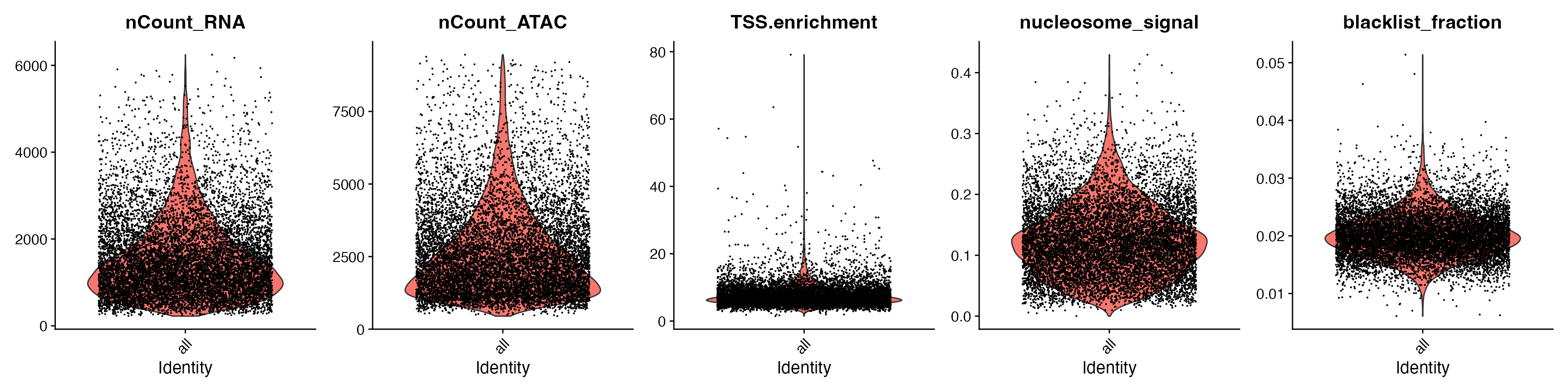
snare <- subset(
  x = snare,
  subset = blacklist_fraction < 0.03 &
    TSS.enrichment < 20 &
    nCount_RNA > 800 &
    nCount_ATAC > 500
)
snare

## An object of class Seurat 
## 277704 features across 8055 samples within 2 assays 
## Active assay: ATAC (244544 features, 0 variable features)
##  2 layers present: counts, data
##  1 other assay present: RNA

Gene expression data processing

Process gene expression data using Seurat

DefaultAssay(snare) <- "RNA"

snare <- FindVariableFeatures(snare, nfeatures = 3000)
snare <- NormalizeData(snare)
snare <- ScaleData(snare)
snare <- RunPCA(snare, npcs = 30)
snare <- RunUMAP(snare, dims = 1:30, reduction.name = "umap.rna")
snare <- FindNeighbors(snare, dims = 1:30)
snare <- FindClusters(snare, resolution = 0.5, algorithm = 3)

## Modularity Optimizer version 1.3.0 by Ludo Waltman and Nees Jan van Eck
## 
## Number of nodes: 8055
## Number of edges: 324240
## 
## Running smart local moving algorithm...
## Maximum modularity in 10 random starts: 0.8900
## Number of communities: 14
## Elapsed time: 4 seconds

p1 <- DimPlot(snare, label = TRUE) + NoLegend() + ggtitle("RNA UMAP")

DNA accessibility data processing

Process the DNA accessibility data using Signac

DefaultAssay(snare) <- 'ATAC'

snare <- FindTopFeatures(snare, min.cutoff = 10)
snare <- RunTFIDF(snare)
snare <- RunSVD(snare)
snare <- RunUMAP(snare, reduction = 'lsi', dims = 2:30, reduction.name = 'umap.atac')
p2 <- DimPlot(snare, reduction = 'umap.atac', label = TRUE) + NoLegend() + ggtitle("ATAC UMAP")

p1 + p2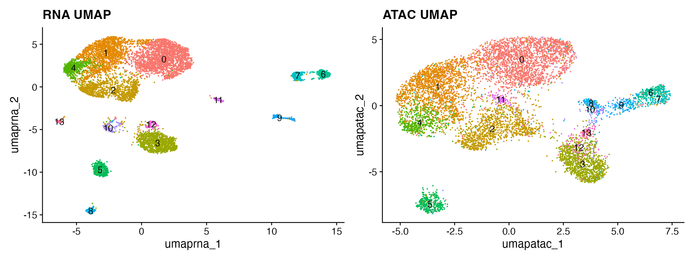

Integration with scRNA-seq data

Next we can annotate cell types in the dataset by transferring labels from an existing scRNA-seq dataset for the adult mouse brain, produced by the Allen Institute.

You can download the raw data for this experiment from the Allen Institute website, and view the code used to construct this object on GitHub. Alternatively, you can download the pre-processed Seurat object here.

# label transfer from Allen brain
allen <- readRDS("../vignette_data/allen_brain.rds")
allen <- UpdateSeuratObject(allen)

# use the RNA assay in the SNARE-seq data for integration with scRNA-seq
DefaultAssay(snare) <- 'RNA'

transfer.anchors <- FindTransferAnchors(
  reference = allen,
  query = snare,
  dims = 1:30,
  reduction = 'cca'
)

predicted.labels <- TransferData(
  anchorset = transfer.anchors,
  refdata = allen$subclass,
  weight.reduction = snare[['pca']],
  dims = 1:30
)

snare <- AddMetaData(object = snare, metadata = predicted.labels)

# label clusters based on predicted ID
new.cluster.ids <- c(
  "L2/3 IT",
  "L4",
  "L6 IT",
  "L5 CT",
  "L4",
  "L5 PT",
  "Pvalb",
  "Sst",
  "Astro",
  "Oligo",
  "Vip/Lamp5",
  "L6 IT.2",
  "L6b",
  "NP"
)
names(x = new.cluster.ids) <- levels(x = snare)
snare <- RenameIdents(object = snare, new.cluster.ids)
snare$celltype <- Idents(snare)
DimPlot(snare, group.by = 'celltype', label = TRUE, reduction = 'umap.rna')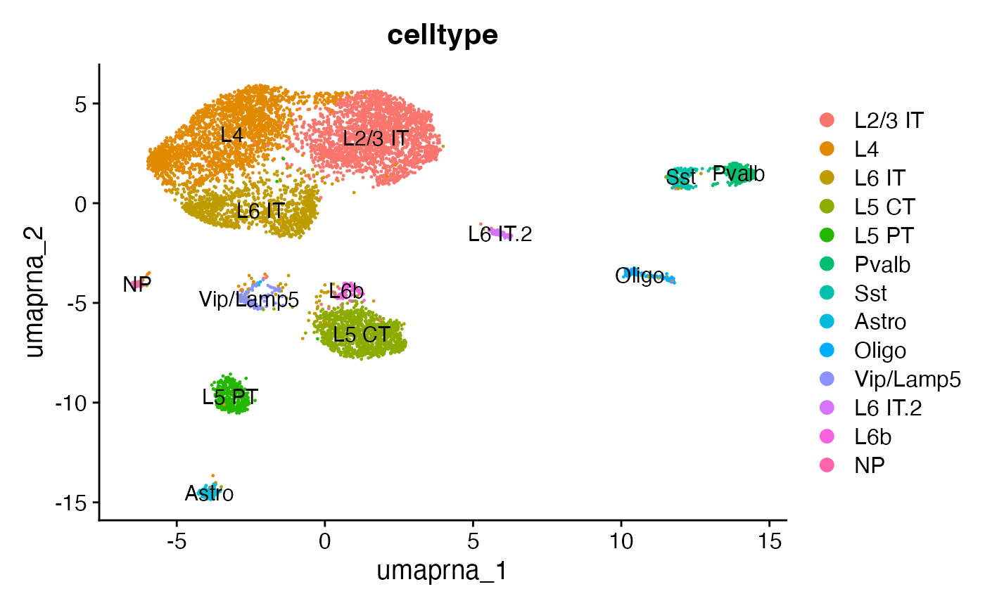

Jointly visualizing gene expression and DNA accessibility

We can visualize both the gene expression and DNA accessibility information at the same time using the CoveragePlot() function. This makes it easy to compare DNA accessibility in a given region for different cell types and overlay gene expression information for different genes.

DefaultAssay(snare) <- "ATAC"
CoveragePlot(snare, region = "chr2-22620000-22660000", features = "Gad2")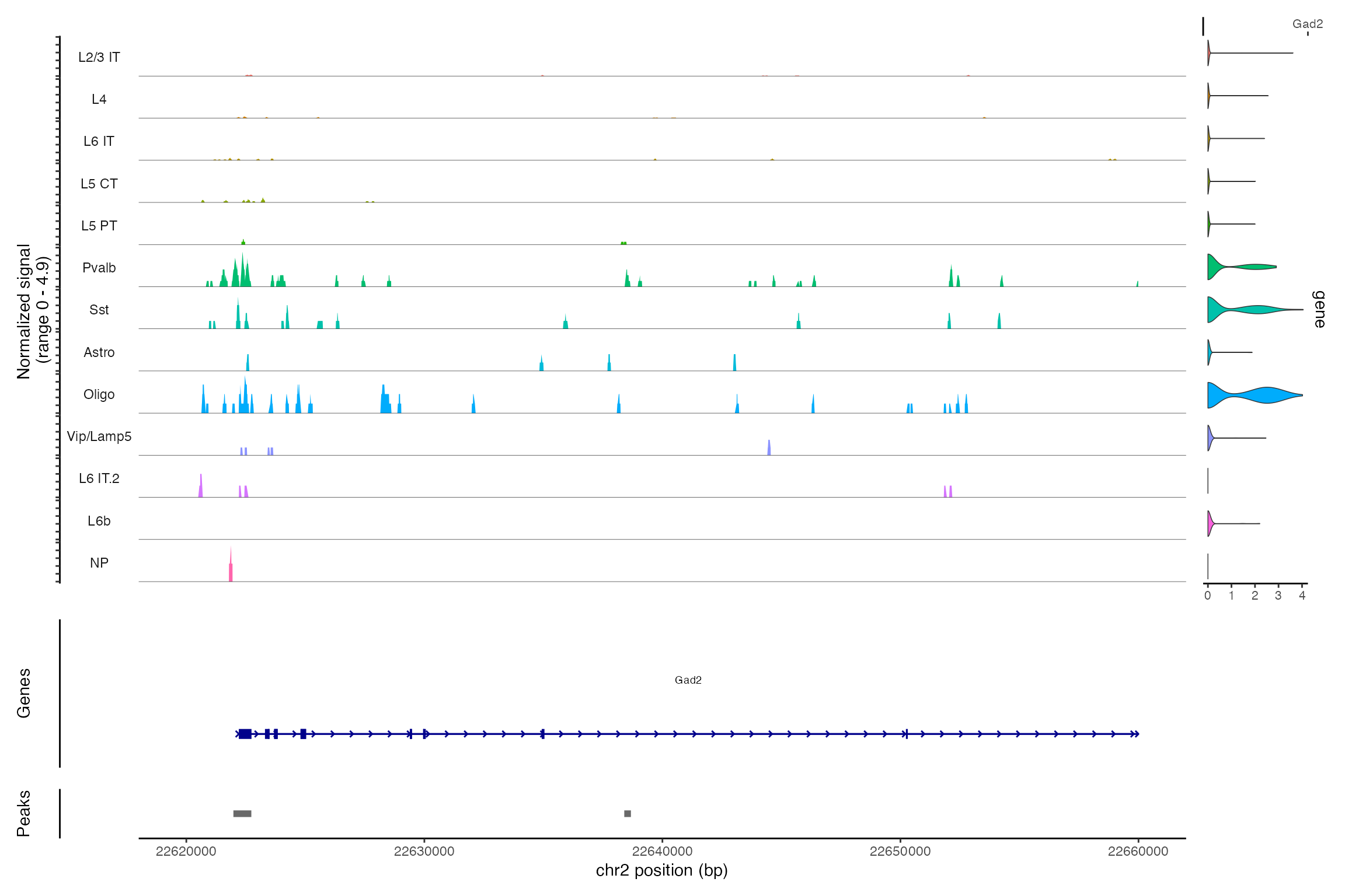

Session Info

sessionInfo()