In this vignette we demonstrate how to merge multiple Seurat objects containing single-cell chromatin data. To demonstrate, we will use four scATAC-seq PBMC datasets provided by 10x Genomics:
View data download code
To download the required data, run the following lines in a shell:
# 500 cell
wget https://cf.10xgenomics.com/samples/cell-atac/1.1.0/atac_pbmc_500_nextgem/atac_pbmc_500_nextgem_fragments.tsv.gz
wget https://cf.10xgenomics.com/samples/cell-atac/1.1.0/atac_pbmc_500_nextgem/atac_pbmc_500_nextgem_fragments.tsv.gz.tbi
wget https://cf.10xgenomics.com/samples/cell-atac/1.1.0/atac_pbmc_500_nextgem/atac_pbmc_500_nextgem_peaks.bed
wget https://cf.10xgenomics.com/samples/cell-atac/1.1.0/atac_pbmc_500_nextgem/atac_pbmc_500_nextgem_singlecell.csv
wget https://cf.10xgenomics.com/samples/cell-atac/1.1.0/atac_pbmc_500_nextgem/atac_pbmc_500_nextgem_filtered_peak_bc_matrix.h5

# 1k cell
wget https://cf.10xgenomics.com/samples/cell-atac/1.1.0/atac_pbmc_1k_nextgem/atac_pbmc_1k_nextgem_fragments.tsv.gz
wget https://cf.10xgenomics.com/samples/cell-atac/1.1.0/atac_pbmc_1k_nextgem/atac_pbmc_1k_nextgem_fragments.tsv.gz.tbi
wget https://cf.10xgenomics.com/samples/cell-atac/1.1.0/atac_pbmc_1k_nextgem/atac_pbmc_1k_nextgem_peaks.bed
wget https://cf.10xgenomics.com/samples/cell-atac/1.1.0/atac_pbmc_1k_nextgem/atac_pbmc_1k_nextgem_singlecell.csv
wget https://cf.10xgenomics.com/samples/cell-atac/1.1.0/atac_pbmc_1k_nextgem/atac_pbmc_1k_nextgem_filtered_peak_bc_matrix.h5

# 5k cell
wget https://cf.10xgenomics.com/samples/cell-atac/1.1.0/atac_pbmc_5k_nextgem/atac_pbmc_5k_nextgem_fragments.tsv.gz
wget https://cf.10xgenomics.com/samples/cell-atac/1.1.0/atac_pbmc_5k_nextgem/atac_pbmc_5k_nextgem_fragments.tsv.gz.tbi
wget https://cf.10xgenomics.com/samples/cell-atac/1.1.0/atac_pbmc_5k_nextgem/atac_pbmc_5k_nextgem_peaks.bed
wget https://cf.10xgenomics.com/samples/cell-atac/1.1.0/atac_pbmc_5k_nextgem/atac_pbmc_5k_nextgem_singlecell.csv
wget https://cf.10xgenomics.com/samples/cell-atac/1.1.0/atac_pbmc_5k_nextgem/atac_pbmc_5k_nextgem_filtered_peak_bc_matrix.h5

# 10k cell
wget https://cf.10xgenomics.com/samples/cell-atac/1.1.0/atac_pbmc_10k_nextgem/atac_pbmc_10k_nextgem_fragments.tsv.gz
wget https://cf.10xgenomics.com/samples/cell-atac/1.1.0/atac_pbmc_10k_nextgem/atac_pbmc_10k_nextgem_fragments.tsv.gz.tbi
wget https://cf.10xgenomics.com/samples/cell-atac/1.1.0/atac_pbmc_10k_nextgem/atac_pbmc_10k_nextgem_peaks.bed
wget https://cf.10xgenomics.com/samples/cell-atac/1.1.0/atac_pbmc_10k_nextgem/atac_pbmc_10k_nextgem_singlecell.csv
wget https://cf.10xgenomics.com/samples/cell-atac/1.1.0/atac_pbmc_10k_nextgem/atac_pbmc_10k_nextgem_filtered_peak_bc_matrix.h5
When merging multiple single-cell chromatin datasets, it’s important to be aware that if peak calling was performed on each dataset independently, the peaks are unlikely to be exactly the same. We therefore need to create a common set of peaks across all the datasets to be merged.
To create a unified set of peaks we can use functions from the GenomicRanges
package. The reduce function from GenomicRanges will merge
all intersecting peaks. Another option is to use the
disjoin function, that will create distinct non-overlapping
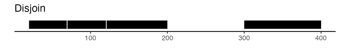
sets of peaks. Here is a visual example to illustrate the difference
between reduce and disjoin:
gr <- GRanges(seqnames = "chr1", ranges = IRanges(start = c(20, 70, 300), end = c(120, 200, 400)))
gr
## GRanges object with 3 ranges and 0 metadata columns:
## seqnames ranges strand
## <Rle> <IRanges> <Rle>
## [1] chr1 20-120 *
## [2] chr1 70-200 *
## [3] chr1 300-400 *
## -------
## seqinfo: 1 sequence from an unspecified genome; no seqlengths## Warning: Using `size` aesthetic for lines was deprecated in ggplot2 3.4.0.
## ℹ Please use `linewidth` instead.
## ℹ The deprecated feature was likely used in the ggbio package.
## Please report the issue at <https://github.com/lawremi/ggbio/issues>.
## This warning is displayed once per session.
## Call `lifecycle::last_lifecycle_warnings()` to see where this warning was
## generated.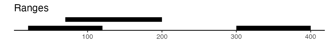

Creating a common peak set
If the peaks were identified independently in each experiment then they will likely not overlap perfectly. We can merge peaks from all the datasets to create a common peak set, and quantify this peak set in each experiment prior to merging the objects.
First we’ll load the peak coordinates for each experiment and convert
them to genomic ranges, the use the GenomicRanges::reduce
function to create a common set of peaks to quantify in each
dataset.
library(Signac)
library(Seurat)
library(GenomicRanges)
library(future)

plan("multicore", workers = 4)
options(future.globals.maxSize = 50000 * 1024^2) # for 50 Gb RAM
# read in peak sets
peaks.500 <- read.table(
  file = "pbmc500/atac_pbmc_500_nextgem_peaks.bed",
  col.names = c("chr", "start", "end")
)
peaks.1k <- read.table(
  file = "pbmc1k/atac_pbmc_1k_nextgem_peaks.bed",
  col.names = c("chr", "start", "end")
)
peaks.5k <- read.table(
  file = "pbmc5k/atac_pbmc_5k_nextgem_peaks.bed",
  col.names = c("chr", "start", "end")
)
peaks.10k <- read.table(
  file = "pbmc10k/atac_pbmc_10k_nextgem_peaks.bed",
  col.names = c("chr", "start", "end")
)

# convert to genomic ranges
gr.500 <- makeGRangesFromDataFrame(peaks.500)
gr.1k <- makeGRangesFromDataFrame(peaks.1k)
gr.5k <- makeGRangesFromDataFrame(peaks.5k)
gr.10k <- makeGRangesFromDataFrame(peaks.10k)

# Create a unified set of peaks to quantify in each dataset
combined.peaks <- reduce(x = c(gr.500, gr.1k, gr.5k, gr.10k))

# Filter out bad peaks based on length
peakwidths <- width(combined.peaks)
combined.peaks <- combined.peaks[peakwidths  < 10000 & peakwidths > 20]
combined.peaks
## GRanges object with 89951 ranges and 0 metadata columns:
## seqnames ranges strand
## <Rle> <IRanges> <Rle>
## [1] chr1 565153-565499 *
## [2] chr1 569185-569620 *
## [3] chr1 713551-714783 *
## [4] chr1 752418-753020 *
## [5] chr1 762249-763345 *
## ... ... ... ...
## [89947] chrY 23422151-23422632 *
## [89948] chrY 23583994-23584463 *
## [89949] chrY 23602466-23602779 *
## [89950] chrY 28816593-28817710 *
## [89951] chrY 58855911-58856251 *
## -------
## seqinfo: 24 sequences from an unspecified genome; no seqlengthsCreate Fragment objects
To quantify our combined set of peaks we’ll need to create a Fragment object for each experiment. The Fragment class is a specialized class defined in Signac to hold all the information related to a single fragment file.
First we’ll load the cell metadata for each experiment so that we
know what cell barcodes are contained in each file, then we can create
Fragment objects using the CreateFragmentObject function.
The CreateFragmentObject function performs some checks to
ensure that the file is present on disk and that it is compressed and
indexed, computes the MD5 sum for the file and the tabix index so that
we can tell if the file is modified at any point, and checks that the
expected cells are present in the file.
# load metadata
md.500 <- read.table(
  file = "pbmc500/atac_pbmc_500_nextgem_singlecell.csv",
  stringsAsFactors = FALSE,
  sep = ",",
  header = TRUE,
  row.names = 1
)[-1, ] # remove the first row

md.1k <- read.table(
  file = "pbmc1k/atac_pbmc_1k_nextgem_singlecell.csv",
  stringsAsFactors = FALSE,
  sep = ",",
  header = TRUE,
  row.names = 1
)[-1, ]

md.5k <- read.table(
  file = "pbmc5k/atac_pbmc_5k_nextgem_singlecell.csv",
  stringsAsFactors = FALSE,
  sep = ",",
  header = TRUE,
  row.names = 1
)[-1, ]

md.10k <- read.table(
  file = "pbmc10k/atac_pbmc_10k_nextgem_singlecell.csv",
  stringsAsFactors = FALSE,
  sep = ",",
  header = TRUE,
  row.names = 1
)[-1, ]

# perform an initial filtering of low count cells
md.500 <- md.500[md.500$passed_filters > 500, ]
md.1k <- md.1k[md.1k$passed_filters > 500, ]
md.5k <- md.5k[md.5k$passed_filters > 500, ]
md.10k <- md.10k[md.10k$passed_filters > 1000, ] # sequenced deeper so set higher cutoff

# create fragment objects
frags.500 <- CreateFragmentObject(
  path = "pbmc500/atac_pbmc_500_nextgem_fragments.tsv.gz",
  cells = rownames(md.500)
)
## Computing hash
frags.1k <- CreateFragmentObject(
  path = "pbmc1k/atac_pbmc_1k_nextgem_fragments.tsv.gz",
  cells = rownames(md.1k)
)
## Computing hash
frags.5k <- CreateFragmentObject(
  path = "pbmc5k/atac_pbmc_5k_nextgem_fragments.tsv.gz",
  cells = rownames(md.5k)
)
## Computing hash
frags.10k <- CreateFragmentObject(
  path = "pbmc10k/atac_pbmc_10k_nextgem_fragments.tsv.gz",
  cells = rownames(md.10k)
)
## Computing hashQuantify peaks in each dataset
We can now create a matrix of peaks x cell for each sample using the
FeatureMatrix function. This function is parallelized using
the future
package. See the parallelization
vignette for more information about using future.
pbmc500.counts <- FeatureMatrix(
  fragments = frags.500,
  features = combined.peaks,
  cells = rownames(md.500)
)

pbmc1k.counts <- FeatureMatrix(
  fragments = frags.1k,
  features = combined.peaks,
  cells = rownames(md.1k)
)

pbmc5k.counts <- FeatureMatrix(
  fragments = frags.5k,
  features = combined.peaks,
  cells = rownames(md.5k)
)

pbmc10k.counts <- FeatureMatrix(
  fragments = frags.10k,
  features = combined.peaks,
  cells = rownames(md.10k)
)
Create the objects
We will now use the quantified matrices to create a Seurat object for each dataset, storing the Fragment object for each dataset in the assay.
pbmc500_assay <- CreateChromatinAssay(pbmc500.counts, fragments = frags.500)
pbmc500 <- CreateSeuratObject(pbmc500_assay, assay = "ATAC", meta.data=md.500)

pbmc1k_assay <- CreateChromatinAssay(pbmc1k.counts, fragments = frags.1k)
pbmc1k <- CreateSeuratObject(pbmc1k_assay, assay = "ATAC", meta.data=md.1k)

pbmc5k_assay <- CreateChromatinAssay(pbmc5k.counts, fragments = frags.5k)
pbmc5k <- CreateSeuratObject(pbmc5k_assay, assay = "ATAC", meta.data=md.5k)

pbmc10k_assay <- CreateChromatinAssay(pbmc10k.counts, fragments = frags.10k)
pbmc10k <- CreateSeuratObject(pbmc10k_assay, assay = "ATAC", meta.data=md.10k)
Merge objects
Now that the objects each contain an assay with the same set of
features, we can use the standard merge function to merge
the objects. This will also merge all the fragment objects so that we
retain the fragment information for each cell in the final merged
object.
# add information to identify dataset of origin
pbmc500$dataset <- 'pbmc500'
pbmc1k$dataset <- 'pbmc1k'
pbmc5k$dataset <- 'pbmc5k'
pbmc10k$dataset <- 'pbmc10k'

# merge all datasets, adding a cell ID to make sure cell names are unique
combined <- merge(
  x = pbmc500,
  y = list(pbmc1k, pbmc5k, pbmc10k),
  add.cell.ids = c("500", "1k", "5k", "10k")
)
combined[["ATAC"]]
## ChromatinAssay data with 89951 features for 21688 cells
## Variable features: 0
## Genome:
## Annotation present: FALSE
## Motifs present: FALSE
## Fragment files: 4
combined <- RunTFIDF(combined)
combined <- FindTopFeatures(combined, min.cutoff = 20)
combined <- RunSVD(combined)
combined <- RunUMAP(combined, dims = 2:50, reduction = 'lsi')
DimPlot(combined, group.by = 'dataset', pt.size = 0.1)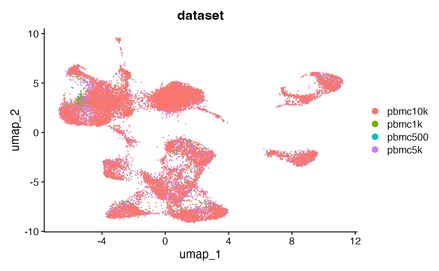
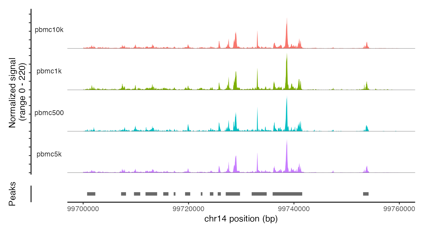
The merged object contains all four fragment objects, and contains an internal mapping of cell names in the object to the cell names in each fragment file so that we can retrieve information from the files without having to change the cell names in each fragment file. We can check that functions that pull data from the fragment files work as expected on the merged object by plotting a region of the genome:
CoveragePlot(
  object = combined,
  group.by = 'dataset',
  region = "chr14-99700000-99760000"
)
Merging without a common feature set
The above approach requires that we have access to a fragment file for each dataset. In some cases we may not have this data (although we can create a fragment file from the BAM file using sinto). In these cases, we can still create a merged object, with the caveat that the resulting merged count matrix may not be as accurate.
The merge function defined in Signac for
ChromatinAssay objects will consider overlapping peaks as
equivalent, and adjust the genomic ranges spanned by the peak so that
the features in each object being merged become equivalent. Note
that this can result in inaccuracies in the count matrix, as some peaks
will be extended to cover regions that were not originally
quantified. This is the best that can be done without
re-quantification, and we recommend always following the procedure
outlined above for object merging whenever possible.
Here we demonstrate merging the same four PBMC datasets without creating a common feature set:
# load the count matrix for each object that was generated by cellranger
counts.500 <- Read10X_h5("pbmc500/atac_pbmc_500_nextgem_filtered_peak_bc_matrix.h5")
counts.1k <- Read10X_h5("pbmc1k/atac_pbmc_1k_nextgem_filtered_peak_bc_matrix.h5")
counts.5k <- Read10X_h5("pbmc5k/atac_pbmc_5k_nextgem_filtered_peak_bc_matrix.h5")
counts.10k <- Read10X_h5("pbmc10k/atac_pbmc_10k_nextgem_filtered_peak_bc_matrix.h5")

# create objects
pbmc500_assay <- CreateChromatinAssay(counts = counts.500, sep = c(":", "-"), min.features = 500)
pbmc500 <- CreateSeuratObject(pbmc500_assay, assay = "peaks")
pbmc1k_assay <- CreateChromatinAssay(counts = counts.1k, sep = c(":", "-"), min.features = 500)
pbmc1k <- CreateSeuratObject(pbmc1k_assay, assay = "peaks")
pbmc5k_assay <- CreateChromatinAssay(counts = counts.5k, sep = c(":", "-"), min.features = 500)
pbmc5k <- CreateSeuratObject(pbmc5k_assay, assay = "peaks")
pbmc10k_assay <- CreateChromatinAssay(counts = counts.10k, sep = c(":", "-"), min.features = 1000)
pbmc10k <- CreateSeuratObject(pbmc10k_assay, assay = "peaks")

# add information to identify dataset of origin
pbmc500$dataset <- 'pbmc500'
pbmc1k$dataset <- 'pbmc1k'
pbmc5k$dataset <- 'pbmc5k'
pbmc10k$dataset <- 'pbmc10k'

# merge
combined <- merge(
  x = pbmc500,
  y = list(pbmc1k, pbmc5k, pbmc10k),
  add.cell.ids = c("500", "1k", "5k", "10k")
)

# process
combined <- RunTFIDF(combined)
combined <- FindTopFeatures(combined, min.cutoff = 20)
combined <- RunSVD(combined)
combined <- RunUMAP(combined, dims = 2:50, reduction = 'lsi')
DimPlot(combined, group.by = 'dataset', pt.size = 0.1)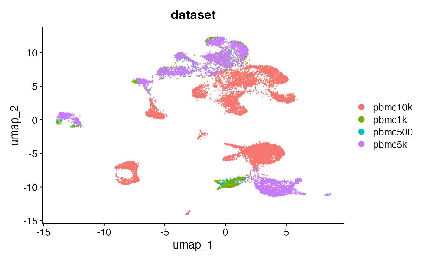
Session Info
## R version 4.5.1 (2025-06-13)
## Platform: aarch64-apple-darwin20
## Running under: macOS Tahoe 26.4
##
## Matrix products: default
## BLAS:   /Library/Frameworks/R.framework/Versions/4.5-arm64/Resources/lib/libRblas.0.dylib
## LAPACK: /Library/Frameworks/R.framework/Versions/4.5-arm64/Resources/lib/libRlapack.dylib;  LAPACK version 3.12.1
##
## locale:
## [1] en_US.UTF-8/en_US.UTF-8/en_US.UTF-8/C/en_US.UTF-8/en_US.UTF-8
##
## time zone: Asia/Singapore
## tzcode source: internal
##
## attached base packages:
## [1] stats4    stats     graphics  grDevices utils     datasets  methods
## [8] base
##
## other attached packages:
##  [1] future_1.70.0           Seurat_5.4.0            SeuratObject_5.3.0.9002
##  [4] sp_2.2-1                Signac_1.17.0           patchwork_1.3.2
##  [7] ggbio_1.58.0            ggplot2_4.0.2           GenomicRanges_1.62.1
## [10] Seqinfo_1.0.0           IRanges_2.44.0          S4Vectors_0.48.0
## [13] BiocGenerics_0.56.0     generics_0.1.4
##
## loaded via a namespace (and not attached):
##   [1] fs_2.0.1                    ProtGenerics_1.42.0
##   [3] matrixStats_1.5.0           spatstat.sparse_3.1-0
##   [5] bitops_1.0-9                httr_1.4.8
##   [7] RColorBrewer_1.1-3          tools_4.5.1
##   [9] sctransform_0.4.3           backports_1.5.0
##  [11] R6_2.6.1                    lazyeval_0.2.2
##  [13] uwot_0.2.4                  withr_3.0.2
##  [15] gridExtra_2.3               progressr_0.18.0
##  [17] cli_3.6.5                   Biobase_2.70.0
##  [19] textshaping_1.0.4           spatstat.explore_3.7-0
##  [21] fastDummies_1.7.5           labeling_0.4.3
##  [23] sass_0.4.10                 S7_0.2.1
##  [25] spatstat.data_3.1-9         ggridges_0.5.7
##  [27] pbapply_1.7-4               pkgdown_2.2.0
##  [29] Rsamtools_2.26.0            systemfonts_1.3.1
##  [31] foreign_0.8-91              dichromat_2.0-0.1
##  [33] parallelly_1.46.1           BSgenome_1.78.0
##  [35] rstudioapi_0.18.0           RSQLite_2.4.6
##  [37] BiocIO_1.20.0               ica_1.0-3
##  [39] spatstat.random_3.4-4       dplyr_1.2.0
##  [41] Matrix_1.7-4                abind_1.4-8
##  [43] lifecycle_1.0.5             yaml_2.3.12
##  [45] SummarizedExperiment_1.40.0 SparseArray_1.10.8
##  [47] Rtsne_0.17                  grid_4.5.1
##  [49] blob_1.3.0                  promises_1.5.0
##  [51] crayon_1.5.3                miniUI_0.1.2
##  [53] lattice_0.22-9              cowplot_1.2.0
##  [55] GenomicFeatures_1.62.0      cigarillo_1.0.0
##  [57] KEGGREST_1.50.0             pillar_1.11.1
##  [59] knitr_1.51                  rjson_0.2.23
##  [61] future.apply_1.20.2         codetools_0.2-20
##  [63] fastmatch_1.1-8             glue_1.8.0
##  [65] spatstat.univar_3.1-6       data.table_1.18.2.1
##  [67] vctrs_0.7.2                 png_0.1-9
##  [69] spam_2.11-3                 gtable_0.3.6
##  [71] cachem_1.1.0                xfun_0.57
##  [73] S4Arrays_1.10.1             mime_0.13
##  [75] survival_3.8-6              RcppRoll_0.3.2
##  [77] fitdistrplus_1.2-6          ROCR_1.0-12
##  [79] nlme_3.1-168                bit64_4.6.0-1
##  [81] RcppAnnoy_0.0.23            GenomeInfoDb_1.46.2
##  [83] bslib_0.10.0                irlba_2.3.7
##  [85] KernSmooth_2.23-26          otel_0.2.0
##  [87] rpart_4.1.24                colorspace_2.1-2
##  [89] DBI_1.3.0                   Hmisc_5.2-5
##  [91] nnet_7.3-20                 tidyselect_1.2.1
##  [93] bit_4.6.0                   compiler_4.5.1
##  [95] curl_7.0.0                  graph_1.88.1
##  [97] htmlTable_2.4.3             hdf5r_1.3.12
##  [99] desc_1.4.3                  DelayedArray_0.36.0
## [101] plotly_4.12.0               stringfish_0.18.0
## [103] rtracklayer_1.70.1          checkmate_2.3.4
## [105] scales_1.4.0                lmtest_0.9-40
## [107] RBGL_1.86.0                 stringr_1.6.0
## [109] digest_0.6.39               goftest_1.2-3
## [111] spatstat.utils_3.2-1        rmarkdown_2.31
## [113] XVector_0.50.0              htmltools_0.5.9
## [115] pkgconfig_2.0.3             base64enc_0.1-6
## [117] sparseMatrixStats_1.22.0    MatrixGenerics_1.22.0
## [119] fastmap_1.2.0               ensembldb_2.34.0
## [121] rlang_1.1.7                 htmlwidgets_1.6.4
## [123] UCSC.utils_1.6.1            shiny_1.13.0
## [125] farver_2.1.2                jquerylib_0.1.4
## [127] zoo_1.8-15                  jsonlite_2.0.0
## [129] BiocParallel_1.44.0         VariantAnnotation_1.56.0
## [131] RCurl_1.98-1.18             magrittr_2.0.4
## [133] Formula_1.2-5               dotCall64_1.2
## [135] Rcpp_1.1.1                  reticulate_1.45.0
## [137] stringi_1.8.7               MASS_7.3-65
## [139] plyr_1.8.9                  parallel_4.5.1
## [141] listenv_0.10.1              ggrepel_0.9.7
## [143] deldir_2.0-4                Biostrings_2.78.0
## [145] splines_4.5.1               tensor_1.5.1
## [147] igraph_2.2.2                spatstat.geom_3.7-0
## [149] RcppHNSW_0.6.0              reshape2_1.4.5
## [151] qs2_0.1.7                   XML_3.99-0.23
## [153] evaluate_1.0.5              biovizBase_1.58.0
## [155] RcppParallel_5.1.11-1       BiocManager_1.30.27
## [157] httpuv_1.6.16               RANN_2.6.2
## [159] tidyr_1.3.2                 purrr_1.2.1
## [161] polyclip_1.10-7             scattermore_1.2
## [163] xtable_1.8-8                restfulr_0.0.16
## [165] AnnotationFilter_1.34.0     RSpectra_0.16-2
## [167] later_1.4.7                 viridisLite_0.4.3
## [169] ragg_1.5.0                  OrganismDbi_1.52.0
## [171] tibble_3.3.1                memoise_2.0.1
## [173] AnnotationDbi_1.72.0        GenomicAlignments_1.46.0
## [175] cluster_2.1.8.2             globals_0.19.1