scATAC-seq data integration

Here we demonstrate the integration of multiple single-cell chromatin datasets derived from human PBMCs. One dataset was generated using the 10x Genomics multiome technology, and includes DNA accessibility and gene expression information for each cell. The other dataset was profiled using 10x Genomics scATAC-seq, and includes DNA accessibility data only.

We will integrate the two datasets together using the shared DNA accessibility assay, using tools available in the Seurat package. Furthermore, we will demonstrate transferring both continuous (gene expression) and categorical (cell labels) information from a reference to a query single-cell chromatin dataset.

View data download code

The PBMC multiome and scATAC-seq data can be downloaded from the 10x website:

# multiome
wget https://cf.10xgenomics.com/samples/cell-arc/1.0.0/pbmc_granulocyte_sorted_10k/pbmc_granulocyte_sorted_10k_filtered_feature_bc_matrix.h5
wget https://cf.10xgenomics.com/samples/cell-arc/1.0.0/pbmc_granulocyte_sorted_10k/pbmc_granulocyte_sorted_10k_atac_fragments.tsv.gz
wget https://cf.10xgenomics.com/samples/cell-arc/1.0.0/pbmc_granulocyte_sorted_10k/pbmc_granulocyte_sorted_10k_atac_fragments.tsv.gz.tbi

# scATAC
# https://www.10xgenomics.com/datasets/10-k-peripheral-blood-mononuclear-cells-pbm-cs-from-a-healthy-donor-next-gem-v-1-1-1-1-standard-2-0-0
wget https://cf.10xgenomics.com/samples/cell-atac/2.0.0/atac_pbmc_10k_nextgem/atac_pbmc_10k_nextgem_fragments.tsv.gz
wget https://cf.10xgenomics.com/samples/cell-atac/2.0.0/atac_pbmc_10k_nextgem/atac_pbmc_10k_nextgem_fragments.tsv.gz.tbi

Preprocessing

Here we’ll load the PBMC multiome data pre-processed in our multiome vignette, and create a new object from the scATAC-seq data:

library(Signac)
library(Seurat)
library(ggplot2)

# load the pre-processed multiome data
pbmc.multi <- readRDS("../vignette_data/pbmc_multiomic.rds")

# process the scATAC data
# first count fragments per cell
fragpath <- "../vignette_data/atac_pbmc_10k_nextgem_fragments.tsv.gz"
fragcounts <- CountFragments(fragments = fragpath)
atac.cells <- fragcounts[fragcounts$frequency_count > 2000, "CB"]

# create the fragment object
atac.frags <- CreateFragmentObject(path = fragpath, cells = atac.cells)

An important first step in any integrative analysis of single-cell chromatin data is to ensure that the same features are measured in each dataset. Here, we quantify the multiome peaks in the ATAC dataset to ensure that there are common features across the two datasets. See the merge vignette for more information about merging chromatin assays.

# quantify multiome peaks in the scATAC-seq dataset
counts <- FeatureMatrix(
  fragments = atac.frags,
  features = granges(pbmc.multi),
  cells = atac.cells
)

# create object
atac.assay <- CreateChromatinAssay(
  counts = counts,
  min.features = 1000,
  fragments = atac.frags
)
pbmc.atac <- CreateSeuratObject(counts = atac.assay, assay = "ATAC")
pbmc.atac <- subset(pbmc.atac, nCount_ATAC > 2000 & nCount_ATAC < 30000)

# compute LSI
pbmc.atac <- FindTopFeatures(pbmc.atac, min.cutoff = 10)
pbmc.atac <- RunTFIDF(pbmc.atac)
pbmc.atac <- RunSVD(pbmc.atac)

Next we can merge the multiome and scATAC datasets together and observe that there is a difference between them that appears to be due to the batch (experiment and technology-specific variation).

# first add dataset-identifying metadata
pbmc.atac$dataset <- "ATAC"
pbmc.multi$dataset <- "Multiome"

# merge
pbmc.combined <- merge(pbmc.atac, pbmc.multi)

# process the combined dataset
pbmc.combined <- FindTopFeatures(pbmc.combined, min.cutoff = 10)
pbmc.combined <- RunTFIDF(pbmc.combined)
pbmc.combined <- RunSVD(pbmc.combined)
pbmc.combined <- RunUMAP(pbmc.combined, reduction = "lsi", dims = 2:30)
p1 <- DimPlot(pbmc.combined, group.by = "dataset")

Integration

To find integration anchors between the two datasets, we need to project them into a shared low-dimensional space. To do this, we’ll use reciprocal LSI projection (projecting each dataset into the others LSI space) by setting reduction="rlsi". For more information about the data integration methods in Seurat, see our recent paper and the Seurat website.

Rather than integrating the normalized data matrix, as is typically done for scRNA-seq data, we’ll integrate the low-dimensional cell embeddings (the LSI coordinates) across the datasets using the IntegrateEmbeddings() function. This is much better suited to scATAC-seq data, as we typically have a very sparse matrix with a large number of features. Note that this requires that we first compute an uncorrected LSI embedding using the merged dataset (as we did above).

# find integration anchors
integration.anchors <- FindIntegrationAnchors(
  object.list = list(pbmc.multi, pbmc.atac),
  anchor.features = rownames(pbmc.multi),
  reduction = "rlsi",
  dims = 2:30
)

# integrate LSI embeddings
integrated <- IntegrateEmbeddings(
  anchorset = integration.anchors,
  reductions = pbmc.combined[["lsi"]],
  new.reduction.name = "integrated_lsi",
  dims.to.integrate = 1:30
)

# create a new UMAP using the integrated embeddings
integrated <- RunUMAP(integrated, reduction = "integrated_lsi", dims = 2:30)
p2 <- DimPlot(integrated, group.by = "dataset")

Finally, we can compare the results of the merged and integrated datasets, and find that the integration has successfully removed the technology-specific variation in the dataset while retaining the cell-type-specific (biological) variation.

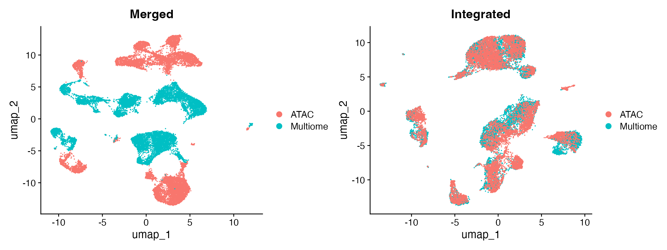
(p1 + ggtitle("Merged")) | (p2 + ggtitle("Integrated"))

Here we’ve demonstrated the integration method using two datasets, but the same workflow can be applied to integrate any number of datasets.

Reference mapping

In cases where we have a large, high-quality dataset, or a dataset containing unique information not present in other datasets (cell type annotations or additional data modalities, for example), we often want to use that dataset as a reference and map queries onto it so that we can interpret these query datasets in the context of the existing reference.

To demonstrate how to do this using single-cell chromatin reference and query datasets, we’ll treat the PBMC multiome dataset here as a reference and map the scATAC-seq dataset to it using the FindTransferAnchors() and MapQuery() functions from Seurat.

# compute UMAP and store the UMAP model
pbmc.multi <- RunUMAP(pbmc.multi, reduction = "lsi", dims = 2:30, return.model = TRUE)

# find transfer anchors
transfer.anchors <- FindTransferAnchors(
  reference = pbmc.multi,
  query = pbmc.atac,
  reference.reduction = "lsi",
  reduction = "lsiproject",
  dims = 2:30
)

# map query onto the reference dataset
pbmc.atac <- MapQuery(
  anchorset = transfer.anchors,
  reference = pbmc.multi,
  query = pbmc.atac,
  refdata = pbmc.multi$predicted.id,
  reference.reduction = "lsi",
  new.reduction.name = "ref.lsi",
  reduction.model = 'umap'
)

What is MapQuery() doing?

MapQuery() is a wrapper function that runs TransferData(), IntegrateEmbeddings(), and ProjectUMAP() for a query dataset, and sets sensible default parameters based on how the anchor object was generated. For finer control over the parameters used by each of these functions, you can pass parameters through MapQuery() to each function using the transferdata.args, integrateembeddings.args, and projectumap.args arguments for MapQuery(), or you can run each of the functions yourself. For example:

pbmc.atac <- TransferData(
  anchorset = transfer.anchors, 
  reference = pbmc.multi,
  weight.reduction = "lsiproject",
  query = pbmc.atac,
  refdata = list(
    celltype = "predicted.id",
    predicted_RNA = "RNA")
)
pbmc.atac <- IntegrateEmbeddings(
  anchorset = transfer.anchors,
  reference = pbmc.multi,
  query = pbmc.atac, 
  reductions = "lsiproject",
  new.reduction.name = "ref.lsi"
)
pbmc.atac <- ProjectUMAP(
  query = pbmc.atac, 
  query.reduction = "ref.lsi",
  reference = pbmc.multi, 
  reference.reduction = "lsi",
  reduction.model = "umap"
)

By running MapQuery(), we have mapped the scATAC-seq dataset onto the the multimodal reference, and enabled cell type labels to be transferred from reference to query. We can visualize these reference mapping results and the cell type labels now associated with the scATAC-seq dataset:

p1 <- DimPlot(pbmc.multi, reduction = "umap", group.by = "predicted.id", label = TRUE, repel = TRUE) + NoLegend() + ggtitle("Reference")
p2 <- DimPlot(pbmc.atac, reduction = "ref.umap", group.by = "predicted.id", label = TRUE, repel = TRUE) + NoLegend() + ggtitle("Query")

p1 | p2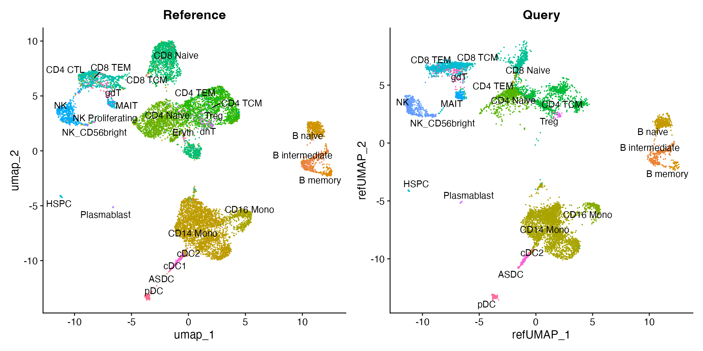

For more information about multimodal reference mapping, see the Seurat vignette.

RNA imputation

Above we transferred categorical information (the cell labels) and mapped the query data onto an existing reference UMAP. We can also transfer continuous data from the reference to the query in the same way. Here we demonstrate transferring the gene expression values from the PBMC multiome dataset (that measured DNA accessibility and gene expression in the same cells) to the PBMC scATAC-seq dataset (that measured DNA accessibility only). Note that we could also transfer these values using the MapQuery() function call above by setting the refdata parameter to a list of values.

# predict gene expression values
rna <- TransferData(
  anchorset = transfer.anchors,
  refdata = LayerData(pbmc.multi, assay = "SCT", layer = "data"),
  weight.reduction = pbmc.atac[["lsi"]],
  dims = 2:30
)

# add predicted values as a new assay
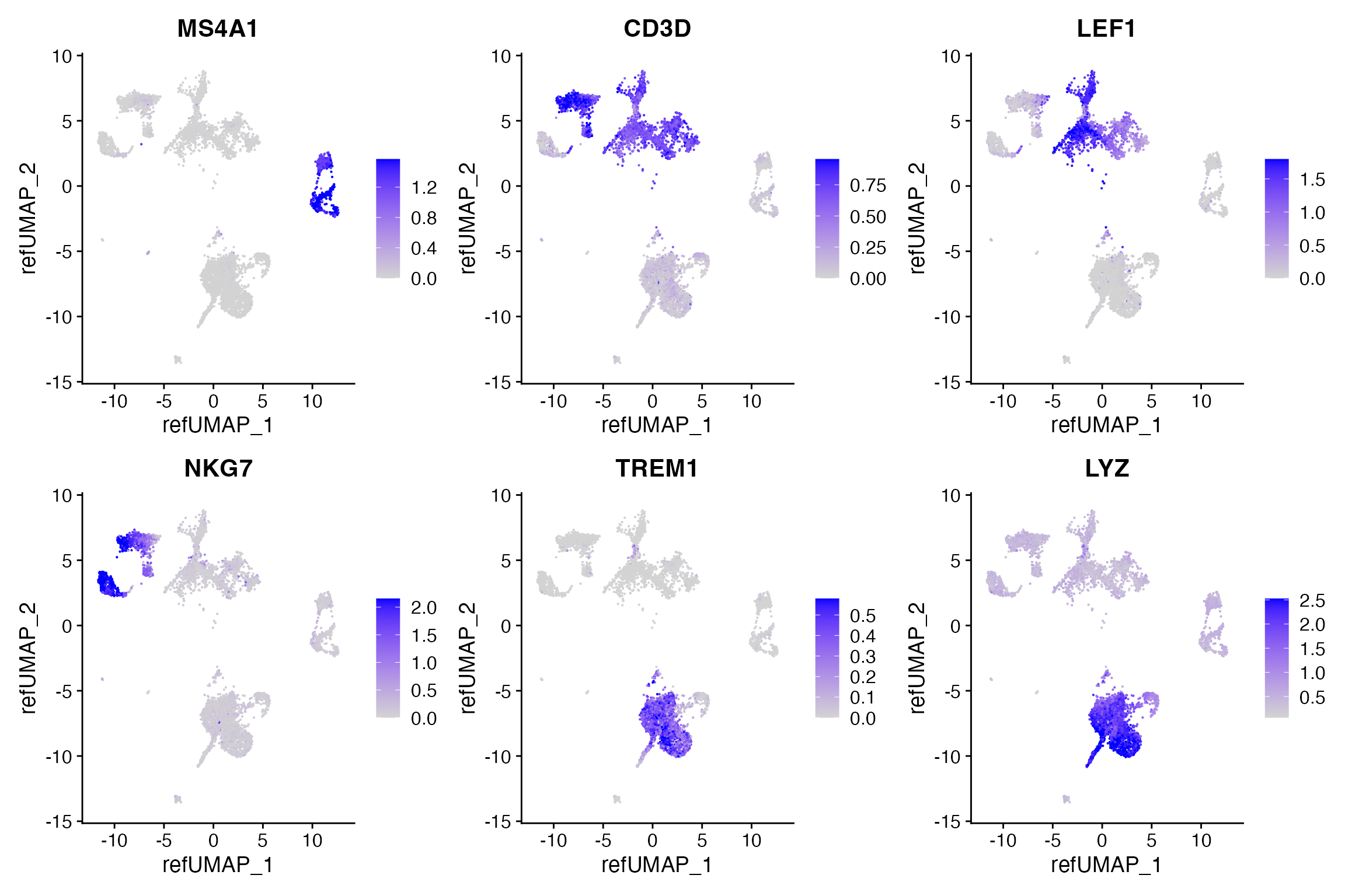
pbmc.atac[["predicted"]] <- rna

We can look at some immune marker genes and see that the predicted expression patterns match our expectation based on known expression patterns.

DefaultAssay(pbmc.atac) <- "predicted"

FeaturePlot(
  object = pbmc.atac,
  features = c('MS4A1', 'CD3D', 'LEF1', 'NKG7', 'TREM1', 'LYZ'),
  pt.size = 0.1,
  max.cutoff = 'q95',
  reduction = "ref.umap",
  ncol = 3
)

Session Info

sessionInfo()

## R version 4.3.1 (2023-06-16)
## Platform: aarch64-apple-darwin20 (64-bit)
## Running under: macOS Sonoma 14.4.1
## 
## Matrix products: default
## BLAS:   /Library/Frameworks/R.framework/Versions/4.3-arm64/Resources/lib/libRblas.0.dylib 
## LAPACK: /Library/Frameworks/R.framework/Versions/4.3-arm64/Resources/lib/libRlapack.dylib;  LAPACK version 3.11.0
## 
## locale:
## [1] C/UTF-8/C/C/C/C
## 
## time zone: Asia/Singapore
## tzcode source: internal
## 
## attached base packages:
## [1] stats     graphics  grDevices utils     datasets  methods   base     
## 
## other attached packages:
## [1] ggplot2_3.5.0      Seurat_5.0.3       SeuratObject_5.0.1 sp_2.1-3          
## [5] Signac_1.13.0     
## 
## loaded via a namespace (and not attached):
##   [1] RColorBrewer_1.1-3      jsonlite_1.8.8          magrittr_2.0.3         
##   [4] spatstat.utils_3.0-4    farver_2.1.1            rmarkdown_2.26         
##   [7] fs_1.6.3                zlibbioc_1.48.0         ragg_1.3.0             
##  [10] vctrs_0.6.5             ROCR_1.0-11             memoise_2.0.1          
##  [13] spatstat.explore_3.2-7  Rsamtools_2.18.0        RCurl_1.98-1.14        
##  [16] RcppRoll_0.3.0          htmltools_0.5.8         sass_0.4.9             
##  [19] sctransform_0.4.1       parallelly_1.37.1       KernSmooth_2.23-22     
##  [22] bslib_0.6.2             htmlwidgets_1.6.4       desc_1.4.3             
##  [25] ica_1.0-3               plyr_1.8.9              plotly_4.10.4          
##  [28] zoo_1.8-12              cachem_1.0.8            igraph_2.0.3           
##  [31] mime_0.12               lifecycle_1.0.4         pkgconfig_2.0.3        
##  [34] Matrix_1.6-5            R6_2.5.1                fastmap_1.1.1          
##  [37] GenomeInfoDbData_1.2.11 fitdistrplus_1.1-11     future_1.33.2          
##  [40] shiny_1.8.1             digest_0.6.35           colorspace_2.1-0       
##  [43] patchwork_1.2.0         S4Vectors_0.40.2        tensor_1.5             
##  [46] RSpectra_0.16-1         irlba_2.3.5.1           textshaping_0.3.7      
##  [49] GenomicRanges_1.54.1    labeling_0.4.3          progressr_0.14.0       
##  [52] spatstat.sparse_3.0-3   fansi_1.0.6             polyclip_1.10-6        
##  [55] abind_1.4-5             httr_1.4.7              compiler_4.3.1         
##  [58] withr_3.0.0             BiocParallel_1.36.0     fastDummies_1.7.3      
##  [61] highr_0.10              MASS_7.3-60.0.1         tools_4.3.1            
##  [64] lmtest_0.9-40           httpuv_1.6.15           future.apply_1.11.2    
##  [67] goftest_1.2-3           glue_1.7.0              nlme_3.1-164           
##  [70] promises_1.2.1          grid_4.3.1              Rtsne_0.17             
##  [73] cluster_2.1.6           reshape2_1.4.4          generics_0.1.3         
##  [76] gtable_0.3.4            spatstat.data_3.0-4     tidyr_1.3.1            
##  [79] data.table_1.15.4       utf8_1.2.4              XVector_0.42.0         
##  [82] spatstat.geom_3.2-9     BiocGenerics_0.48.1     RcppAnnoy_0.0.22       
##  [85] ggrepel_0.9.5           RANN_2.6.1              pillar_1.9.0           
##  [88] stringr_1.5.1           spam_2.10-0             RcppHNSW_0.6.0         
##  [91] later_1.3.2             splines_4.3.1           dplyr_1.1.4            
##  [94] lattice_0.22-6          deldir_2.0-4            survival_3.5-8         
##  [97] tidyselect_1.2.1        Biostrings_2.70.2       miniUI_0.1.1.1         
## [100] pbapply_1.7-2           knitr_1.45              gridExtra_2.3          
## [103] IRanges_2.36.0          scattermore_1.2         stats4_4.3.1           
## [106] xfun_0.43               matrixStats_1.2.0       stringi_1.8.3          
## [109] lazyeval_0.2.2          yaml_2.3.8              evaluate_0.23          
## [112] codetools_0.2-19        tibble_3.2.1            cli_3.6.2              
## [115] uwot_0.1.16             xtable_1.8-4            reticulate_1.35.0      
## [118] systemfonts_1.0.6       munsell_0.5.0           jquerylib_0.1.4        
## [121] Rcpp_1.0.12             GenomeInfoDb_1.38.7     spatstat.random_3.2-3  
## [124] globals_0.16.3          png_0.1-8               parallel_4.3.1         
## [127] pkgdown_2.0.7           dotCall64_1.1-1         bitops_1.0-7           
## [130] listenv_0.9.1           viridisLite_0.4.2       scales_1.3.0           
## [133] ggridges_0.5.6          leiden_0.4.3.1          purrr_1.0.2            
## [136] crayon_1.5.2            rlang_1.1.3             cowplot_1.1.3          
## [139] fastmatch_1.1-4

Compiled: April 04, 2024

Preprocessing

Integration

Reference mapping

RNA imputation