Finding co-accessible networks with Cicero
Compiled: April 01, 2026
Source:vignettes/cicero.Rmd
cicero.RmdIn this vignette we will demonstrate how to find cis-co-accessible networks with Cicero using single-cell ATAC-seq data. Please see the Cicero website for information about Cicero.
To facilitate conversion between the Seurat (used by Signac) and CellDataSet (used by Cicero) formats, we will use a conversion function in the SeuratWrappers package available on GitHub.
Data loading
We will use a single-cell ATAC-seq dataset containing human CD34+ hematopoietic stem and progenitor cells published by Satpathy and Granja et al. (2019, Nature Biotechnology). The processed datasets are available on NCBI GEO here: https://www.ncbi.nlm.nih.gov/geo/query/acc.cgi?acc=GSE129785
This is the same dataset we used in the trajectory vignette, and we’ll start by loading the dataset that was created in that vignette. See the trajectory vignette for the code used to create the object from raw data.
First we will load their dataset and perform some standard preprocessing using Signac.
# load the object created in the Monocle 3 vignette
bone <- qs2::qs_read("cd34.qs2")
Create the Cicero object
We can find cis-co-accessible networks (CCANs) using Cicero.
The Cicero developers have developed a separate branch of the package
that works with a Monocle 3 CellDataSet object. We will
first make sure this branch is installed, then convert our
Seurat object for the whole bone marrow dataset to
CellDataSet format.
# Install Cicero
if (!requireNamespace("remotes", quietly = TRUE))
    install.packages("remotes")
remotes::install_github("cole-trapnell-lab/cicero-release", ref = "monocle3")
## png (0.1-8 -> 0.1-9 ) [CRAN]
## fs (1.6.6 -> 2.0.1 ) [CRAN]
## RCurl (1.98-1.17 -> 1.98-1.18) [CRAN]
## XML (3.99-0.22 -> 3.99-0.23) [CRAN]
## tinytex (0.58 -> 0.59 ) [CRAN]
## xfun (0.56 -> 0.57 ) [CRAN]
## highr (0.11 -> 0.12 ) [CRAN]
## rmarkdown (2.30 -> 2.31 ) [CRAN]##
## The downloaded binary packages are in
## /var/folders/n5/1l8rdp0951gcwznhr_sxwj0m0000gp/T//RtmpVfe2dz/downloaded_packages
## ── R CMD build ─────────────────────────────────────────────────────────────────
## * checking for file ‘/private/var/folders/n5/1l8rdp0951gcwznhr_sxwj0m0000gp/T/RtmpVfe2dz/remotescf662e9d66d2/cole-trapnell-lab-cicero-release-495ef0d/DESCRIPTION’ ... OK
## * preparing ‘cicero’:
## * checking DESCRIPTION meta-information ... OK
## * checking for LF line-endings in source and make files and shell scripts
## * checking for empty or unneeded directories
## * looking to see if a ‘data/datalist’ file should be added
## * building ‘cicero_1.3.9.tar.gz’
library(cicero)
# convert to CellDataSet format and make the cicero object
bone.cds <- as.cell_data_set(x = bone)
bone.cicero <- make_cicero_cds(bone.cds, reduced_coordinates = reducedDims(bone.cds)$UMAP)
Find Cicero connections
We’ll demonstrate running Cicero here using just one chromosome to save some time, but the same workflow can be applied to find CCANs for the whole genome.
Here we demonstrate the most basic workflow for running Cicero. This workflow can be broken down into several steps, each with parameters that can be changed from their defaults to fine-tune the Cicero algorithm depending on your data. We highly recommend that you explore the Cicero website, paper, and documentation for more information.
# get the chromosome sizes from the Seurat object
genome <- seqlengths(bone)

# use chromosome 1 to save some time
# omit this step to run on the whole genome
genome <- genome[1]

# convert chromosome sizes to a dataframe
genome.df <- data.frame("chr" = names(genome), "length" = genome)

# run cicero
conns <- run_cicero(bone.cicero, genomic_coords = genome.df, sample_num = 100)
## [1] "Starting Cicero"
## [1] "Calculating distance_parameter value"
## [1] "Running models"
## [1] "Assembling connections"
## [1] "Successful cicero models: 755"
## [1] "Other models: "
##
## Too many elements in range Zero or one element in range
## 157 86
## [1] "Models with errors: 0"
## [1] "Done"
head(conns)## Peak1 Peak2 coaccess
## 1 chr1-100003337-100003837 chr1-99791719-99792219 0
## 2 chr1-100003337-100003837 chr1-99828699-99829199 0
## 3 chr1-100003337-100003837 chr1-99835542-99836042 0
## 4 chr1-100003337-100003837 chr1-99836217-99836717 0
## 5 chr1-100003337-100003837 chr1-99839576-99840076 0
## 6 chr1-100003337-100003837 chr1-99840640-99841140 0Find cis-co-accessible networks (CCANs)
Now that we’ve found pairwise co-accessibility scores for each peak,
we can now group these pairwise connections into larger co-accessible
networks using the generate_ccans() function from
Cicero.
ccans <- generate_ccans(conns)## [1] "Coaccessibility cutoff used: 0.22"
head(ccans)## Peak CCAN
## chr1-10009702-10010202 chr1-10009702-10010202 1
## chr1-100151188-100151688 chr1-100151188-100151688 2
## chr1-100165566-100166066 chr1-100165566-100166066 2
## chr1-100247892-100248392 chr1-100247892-100248392 2
## chr1-100252210-100252710 chr1-100252210-100252710 4
## chr1-100259383-100259883 chr1-100259383-100259883 4Add links to a Seurat object
We can add the co-accessible links found by Cicero to the
ChromatinAssay object in Seurat. Using the
ConnectionsToLinks() function in Signac we can convert the
outputs of Cicero to the format needed to store in the
links slot in the ChromatinAssay, and add this
to the object using the Links<- assignment function.
links <- ConnectionsToLinks(conns = conns, ccans = ccans)
Links(bone) <- links
We can now visualize these links along with DNA accessibility
information by running CoveragePlot() for a region:
CoveragePlot(bone, region = "chr1-40189344-40252549")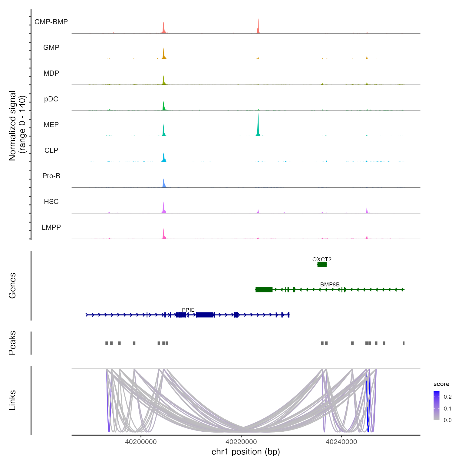
Acknowledgements
Thanks to the developers of Cicero, especially Cole Trapnell, Hannah Pliner, and members of the Trapnell lab. If you use Cicero please cite the Cicero paper.
Session Info
## R version 4.5.1 (2025-06-13)
## Platform: aarch64-apple-darwin20
## Running under: macOS Tahoe 26.4
##
## Matrix products: default
## BLAS:   /Library/Frameworks/R.framework/Versions/4.5-arm64/Resources/lib/libRblas.0.dylib
## LAPACK: /Library/Frameworks/R.framework/Versions/4.5-arm64/Resources/lib/libRlapack.dylib;  LAPACK version 3.12.1
##
## locale:
## [1] en_US.UTF-8/en_US.UTF-8/en_US.UTF-8/C/en_US.UTF-8/en_US.UTF-8
##
## time zone: Asia/Singapore
## tzcode source: internal
##
## attached base packages:
## [1] grid      stats4    stats     graphics  grDevices utils     datasets
## [8] methods   base
##
## other attached packages:
##  [1] cicero_1.3.9                Gviz_1.54.0
##  [3] monocle3_1.4.26             SingleCellExperiment_1.32.0
##  [5] SummarizedExperiment_1.40.0 GenomicRanges_1.62.1
##  [7] Seqinfo_1.0.0               IRanges_2.44.0
##  [9] S4Vectors_0.48.0            MatrixGenerics_1.22.0
## [11] matrixStats_1.5.0           Biobase_2.70.0
## [13] BiocGenerics_0.56.0         generics_0.1.4
## [15] patchwork_1.3.2             ggplot2_4.0.2
## [17] SeuratWrappers_0.4.0        Seurat_5.4.0
## [19] SeuratObject_5.3.0.9002     sp_2.2-1
## [21] Signac_1.17.0
##
## loaded via a namespace (and not attached):
##   [1] R.methodsS3_1.8.2        dichromat_2.0-0.1        progress_1.2.3
##   [4] nnet_7.3-20              goftest_1.2-3            Biostrings_2.78.0
##   [7] vctrs_0.7.2              spatstat.random_3.4-4    digest_0.6.39
##  [10] png_0.1-8                ggrepel_0.9.7            deldir_2.0-4
##  [13] parallelly_1.46.1        combinat_0.0-8           MASS_7.3-65
##  [16] pkgdown_2.2.0            reshape2_1.4.5           httpuv_1.6.16
##  [19] withr_3.0.2              xfun_0.56                survival_3.8-6
##  [22] memoise_2.0.1            systemfonts_1.3.1        ragg_1.5.0
##  [25] zoo_1.8-15               pbapply_1.7-4            R.oo_1.27.1
##  [28] Formula_1.2-5            prettyunits_1.2.0        KEGGREST_1.50.0
##  [31] promises_1.5.0           otel_0.2.0               httr_1.4.8
##  [34] restfulr_0.0.16          globals_0.19.1           fitdistrplus_1.2-6
##  [37] ps_1.9.1                 stringfish_0.18.0        rstudioapi_0.18.0
##  [40] UCSC.utils_1.6.1         miniUI_0.1.2             processx_3.8.6
##  [43] base64enc_0.1-6          curl_7.0.0               polyclip_1.10-7
##  [46] SparseArray_1.10.8       xtable_1.8-8             stringr_1.6.0
##  [49] desc_1.4.3               evaluate_1.0.5           S4Arrays_1.10.1
##  [52] BiocFileCache_3.0.0      hms_1.1.4                irlba_2.3.7
##  [55] colorspace_2.1-2         filelock_1.0.3           ROCR_1.0-12
##  [58] qs2_0.1.7                reticulate_1.45.0        spatstat.data_3.1-9
##  [61] magrittr_2.0.4           lmtest_0.9-40            later_1.4.7
##  [64] viridis_0.6.5            lattice_0.22-9           spatstat.geom_3.7-0
##  [67] future.apply_1.20.2      scattermore_1.2          XML_3.99-0.22
##  [70] cowplot_1.2.0            RcppAnnoy_0.0.23         Hmisc_5.2-5
##  [73] pillar_1.11.1            nlme_3.1-168             compiler_4.5.1
##  [76] RSpectra_0.16-2          stringi_1.8.7            tensor_1.5.1
##  [79] minqa_1.2.8              GenomicAlignments_1.46.0 plyr_1.8.9
##  [82] crayon_1.5.3             abind_1.4-8              BiocIO_1.20.0
##  [85] bit_4.6.0                dplyr_1.2.0              fastmatch_1.1-8
##  [88] codetools_0.2-20         textshaping_1.0.4        bslib_0.10.0
##  [91] slam_0.1-55              biovizBase_1.58.0        plotly_4.12.0
##  [94] monocle_2.38.0           mime_0.13                leidenbase_0.1.36
##  [97] splines_4.5.1            Rcpp_1.1.1               fastDummies_1.7.5
## [100] dbplyr_2.5.2             sparseMatrixStats_1.22.0 interp_1.1-6
## [103] knitr_1.51               blob_1.3.0               AnnotationFilter_1.34.0
## [106] lme4_1.1-38              fs_1.6.6                 listenv_0.10.1
## [109] checkmate_2.3.4          Rdpack_2.6.6             pkgbuild_1.4.8
## [112] tibble_3.3.1             Matrix_1.7-4             callr_3.7.6
## [115] statmod_1.5.1            tweenr_2.0.3             pkgconfig_2.0.3
## [118] pheatmap_1.0.13          tools_4.5.1              cachem_1.1.0
## [121] rbibutils_2.4.1          cigarillo_1.0.0          RSQLite_2.4.6
## [124] viridisLite_0.4.3        DBI_1.3.0                fastmap_1.2.0
## [127] rmarkdown_2.30           scales_1.4.0             ica_1.0-3
## [130] Rsamtools_2.26.0         sass_0.4.10              FNN_1.1.4.1
## [133] BiocManager_1.30.27      dotCall64_1.2            VariantAnnotation_1.56.0
## [136] RANN_2.6.2               rpart_4.1.24             farver_2.1.2
## [139] reformulas_0.4.4         yaml_2.3.12              VGAM_1.1-14
## [142] latticeExtra_0.6-31      foreign_0.8-91           rtracklayer_1.70.1
## [145] cli_3.6.5                purrr_1.2.1              lifecycle_1.0.5
## [148] uwot_0.2.4               backports_1.5.0          BiocParallel_1.44.0
## [151] gtable_0.3.6             rjson_0.2.23             ggridges_0.5.7
## [154] progressr_0.18.0         parallel_4.5.1           limma_3.66.0
## [157] jsonlite_2.0.0           RcppHNSW_0.6.0           bitops_1.0-9
## [160] assertthat_0.2.1         bit64_4.6.0-1            Rtsne_0.17
## [163] spatstat.utils_3.2-1     RcppParallel_5.1.11-1    jquerylib_0.1.4
## [166] spatstat.univar_3.1-6    R.utils_2.13.0           lazyeval_0.2.2
## [169] shiny_1.13.0             htmltools_0.5.9          DDRTree_0.1.6
## [172] sctransform_0.4.3        rappdirs_0.3.4           ensembldb_2.34.0
## [175] glue_1.8.0               spam_2.11-3              httr2_1.2.2
## [178] XVector_0.50.0           RCurl_1.98-1.17          BSgenome_1.78.0
## [181] jpeg_0.1-11              gridExtra_2.3            boot_1.3-32
## [184] igraph_2.2.2             R6_2.6.1                 tidyr_1.3.2
## [187] labeling_0.4.3           RcppRoll_0.3.2           HSMMSingleCell_1.30.0
## [190] GenomicFeatures_1.62.0   cluster_2.1.8.2          GenomeInfoDb_1.46.2
## [193] nloptr_2.2.1             DelayedArray_0.36.0      tidyselect_1.2.1
## [196] ProtGenerics_1.42.0      htmlTable_2.4.3          ggforce_0.5.0
## [199] AnnotationDbi_1.72.0     future_1.70.0            fastICA_1.2-7
## [202] rsvd_1.0.5               KernSmooth_2.23-26       S7_0.2.1
## [205] data.table_1.18.2.1      htmlwidgets_1.6.4        RColorBrewer_1.1-3
## [208] biomaRt_2.66.1           rlang_1.1.7              spatstat.sparse_3.1-0
## [211] spatstat.explore_3.7-0   remotes_2.5.0